
Damped Springs
I've worked on third-person camera systems for numerous games and I often need a method for smoothing camera motion as the player moves through the world. The player’s motion may create sharp, discontinuous changes in direction, speed or even position. The camera, however, should:
- Avoid discontinuities in motion. Accelerate and decelerate as needed rather than snap to a new velocity.
- Never let the player outrun the camera. The farther away he gets, the faster the camera needs to move.
- Move exactly the same with respect to time regardless of frame rate.
To solve this problem, I often simulate the camera with a set of damped springs.
If the camera needs to remain a constant distance from the player (e.g. a Mario style camera), I can use a spring for its radial distance. If the camera position is fixed in space and it rotates around to track the player, I can simulate springs for pitch and yaw.
Now that we have some context, let’s dive into the details and work towards being able to write a function that can integrate the motion of a damped spring. I'm going to try and cover the full derivation of the damped harmonic motion formulas for those interested, but be warned that there is a lot of math. If you just want to grab the code, feel free to skip ahead to the last page.
Simple Harmonic Motion
Before we get into damped springs, I’m going to talk about normal springs. We will derive the equations of motion for a normal spring with the same approach that we will use for damped springs. This will help us learn some of math involved with simpler equations.
Your everyday spring system moves according to simple harmonic motion. I’m sure you are familiar with how a spring behaves, but let’s spell it out anyways for the sake of completeness. If you hold a small coiled metal spring in your hand, it will remain at some rest length. If you try to compress the spring, it will apply a force trying to grow back to its rest length. If you stretch the spring, it will apply a force trying to shrink back to its rest length. We call this rest length, the equilibrium position of the spring. Unlike a real world coiled spring, our simple harmonic motion spring will have no drag, friction or other complex forces on it. It only has the push and pull due to fighting compression or extension.
Another interesting property of springs is that the farther you compress or stretch them from their equilibrium position, the more force they will apply. According to the needs of the camera example I started with, this is great because the camera will move back to the player faster if it starts to drag behind.
Let’s pretend one end of our spring is rigidly fixed to the position zero and a point mass is attached to the other end (e.g. our camera). At rest, the spring has a length, \(r\). As the current length, \(p\), deviates farther from \(r\), we will generate a force in the opposite direction. We can define this force as:
\(F=-k(p-r)\)
The value, \(k\), is called the spring constant and controls how strong the spring is. Higher values of \(k\) will create a stronger force for the same displacement from the equilibrium position, \(r\) .
In order to make our lives easier, let’s define the variable, \(x\), to be the position relative to equilibrium and simplify the force equation.
\(x = p - r\)
\(F = -kx\)
Ordinary Differential Equation
As stated before, we really want damped harmonic motion, but it will be a useful exercise to learn how we derive the formulas for simple harmonic motion first. We will also learn why a simple harmonic oscillator (the spring) is not sufficient for the needs of a simulated video game camera.
Our goal is to find a function \(x(t)\) that solves our position, \(x\), based on time, \(t\).
If you recall your physics, acceleration is the derivative of velocity and velocity is the derivative of position. I will refer to the position, velocity and acceleration of our equilibrium relative position, \(x\) , as follows.
\(x = position\)
\(v = {dx \over dt} = velocity\)
\(a = {dv \over dt} = acceleration\)
The next prerequisite before we can continue is Newton’s second law of motion. That’s the one that says that the acceleration induced by a force is inversely proportional to mass (i.e. massive rocks are hard to push). This is also the law that gives us the equation \(F = ma\), where \(m\) is the mass of our object attached to the spring.
Earlier we said that force was equivalent to \(-kx\) due to the spring. We can combine these force equations into one equality as follows:
\(F =ma\)
\(F = -kx\)
\(ma = -kx\)
\(ma + kx = 0\)
In order to simplify the remaining math, we are going rearrange the equation and define a new variable, \(\omega\). We will later find that \(\omega\) is the angular frequency of the spring.
\(a + {k \over m}x = 0\)
\(\omega = \sqrt{k \over m}\)
\(a + \omega^2 x = 0\)
This equation says that our position is dependent upon our acceleration and vice versa. It is called an ordinary differential equation (ODE). An ODE is an equation containing the derivatives of a single independent variable. In our case this variable is x and its second derivative a. Our ODE is also considered linear and homogenous. It is a linear ODE because all of its derivatives have an exponent of one. It is a homogenous ODE because the sum of all the terms containing \(x\) and its derivates is equal to zero (i.e. there is no remaining constant term).
Because the highest derivative in our linear ODE is the second derivative, it is considered to be of second degree. The degree of a linear ODE determines how many linearly independent solutions it has. These linearly independent solutions create a basis for a solution vector space in which any scaled combination is also a solution. For example, if \(s_1\) and \(s_2\) are two linearly independent solutions to the system, then \(3s_1 + 5 s_2\) is also a solution to the system. This means that there are an infinite number of solutions but they are all constrained within the vector space.
I'm not going to go into too much detail about what make a set of solutions linearly independent or how to test their independence, but if you are familiar with linear algebra you can imaging an n-dimensional vector where n is the degree of the ODE (in our case it is 2). The elements of the vector are a solution and its derivatives up to the nth degree. Our solution basis is a set of these vectors - one for each solution. For the basis to be linearly independent, you should not be able to derive any one vector as a scaled combination of the others.
The ODE's degree also determines how many initial conditions must be specified to solve a particular solution. This makes sense for a point mass attached to a spring. When simulating the spring, we will need to specify our initial spring position and initial spring velocity. Those are the two initial conditions that determine how the system will behave over time.
Before we can input our initial position and velocity, we need to solve an equation for the general motion of the system.
General Solution
\({d \over dy} e^u = {du \over dy} e^u\)
If we let \(x\) equal \(e^{z t}\), we can simplify as follows
\(x = e^{z t}\)
\(v = {dx \over dt} = ze^{z t}\)
\(a = {dv \over dt} = z^2 e^{z t}\)
\(a + \omega^2 x = 0\)
\(z^2 e^{z t} + \omega^2 e^{z t} = 0\)
\((z^2 + \omega^2) e^{z t} = 0\)
Dividing both sides by \(e ^ {z t}\) gives us the characteristic equation:
\(z^2 + \omega^2 = 0\)
In order to solve for \(z\), we can rearrange the equation and factor into a difference of squares. To do this, we make use of the imaginary unit, \(i\), which is equal to the \(\sqrt{-1}\)
\(z^2 - i^2 \omega^2 = 0\)
\((z + i \omega) (z - i \omega) = 0\)
The factored equation shows us two possible solutions for \(z\)
\(z_1 = -i \omega\)
\(z_2 = i \omega\)
By substituting \(z\) back into our original equations for \(x\), we get
\(x_1 = e ^ {z_1 t} = e ^ {-i \omega t}\)
\(x_2 = e ^ {z_2 t} = e ^ {i \omega t}\)
If you recall, we determined that our equation, \(ma + kx = 0\), was a linear ODE and thus any linear combination of solutions is also a solution. This lets us combine our two solutions for \(x\) into one equation representing the general solution for \(x(t)\). The variables \(c_1\) and \(c_2\) will be used as linear scalars for each solution.
\(x(t) = c_1 x_1 + c_2 x_2\)
\(x(t) = c_1 e ^ {-i \omega t} + c_2 e ^ {i \omega t}\)
Using Euler’s formula, \(e^{i y} = \cos (y) + i \sin (y)\), we can convert to a trigonometric equation
\(x(t) = c_1 \Big( \cos(-\omega t) + i \sin(-\omega t) \Big) + c_2 \Big( \cos(\omega t) + i \sin(\omega t) \Big)\)
Using the trigonometric identities \(\cos(-\theta) = \cos(\theta)\) and \(\sin(-\theta) = -\sin(\theta)\), let’s simplify and regroup terms.
\(x(t) = c_1 \Big( cos(\omega t) - i sin(\omega t) \Big) + c_2 \Big( \cos(w t) + i \sin(\omega t) \Big)\)
\(x(t) = (c_1 + c_2) \cos(\omega t) + i (c_2 - c_1) \sin(\omega t)\)
By taking the derivative with respect to \(t\), we can solve for \(v(t)\)
\(v(t) = -\omega (c1 + c2) \sin(\omega t) + i \omega (c2 - c1) \cos(\omega t)\)
Particular Solution
The terms \(c1\) and \(c2\) are arbitrary constant scalars that select from an infinite number of solutions to the original equation, \(a + \omega^2 x = 0\). We can derive their values based on the initial state of the spring to generate a particular solution.
First, we solve \(x\) for a time value of \(t=0\).
\(x(0) = (c_1 + c_2) \cos(\omega 0) + i (c_2 - c_1) \sin(\omega 0)\)
\(x(0) = (c_1 + c_2)\)
Next, we solve \(v(t)\) for a time value of \(t=0\).
\(v(0) = -\omega (c_1 + c_2) \sin(w 0) + i \omega (c_2 - c_1) \cos(w 0)\)
\(v(0) = i \omega (c_2 - c_1)\)
Based on the \(x(0)\) and \(v(0)\) equations, we can solve for the \((c_1 + c_2)\) and \((c_2 - c_1)\) terms. Let's also let \(x_0 = x(0)\) and \(v_0 = v(0)\) to simplify the equations a bit.
\((c_1 + c_2) = x_0\)
\((c_2 - c_1) = {v_0 \over i \omega}\)
Now substitute the values for \((c_1 + c_2)\) and \((c_2 - c_1)\) back into the equation for \(x(t)\).
\(x(t) = x_0 \cos(\omega t) + i {v_0 \over i \omega} \sin(\omega t)\)
\(x(t) = x_0 \cos(\omega t) + {v_0 \over \omega} \sin(\omega t)\)
Next we do the same for\(v(t)\).
\(v(t) = -\omega x_0 \sin(w t) + i \omega {v_0 \over i \omega} \cos(\omega t)\)
\(v(t) = -w x_0 \sin(\omega t) + v_0 \cos(\omega t)\)
Using our equations for \(x(t)\) and \(v(t)\), we can simulate simple harmonic motion over an elapsed period of time. For example, let's consider the case where we are simulating the yaw rotation of a camera over a single game frame.
- Let \(k\) be our spring constant.
- Let \(m\) be our spring point mass.
- Let \(x_0\) be our current distance from the desired yaw angle (chosen to be the shortest angle around the circle).
- Let \(v_0\) be our current yaw-velocity.
- Let \(t\) be the duration of the game frame.
- Let \(x(t)\) be our new distance from the desired yaw angle.
- Let \(v(t)\) be our new yaw-velocity.
We can compute our new yaw-position and yaw-velocity by running the following equations.
\(\omega = \sqrt{k \over m}\)
\(x(t) = x_0 \cos(\omega t) + {v_0 \over \omega} \sin(\omega t)\)
\(v(t) = -w x_0 \sin(\omega t) + v_0 \cos(\omega t)\)
Instead of having the user specify \(k\) and \(m\), it might be more useful to only define \(\omega\) which turns out to correspond to the angular frequency of the ocillation. This means that choosing higher values for \(\omega\) will create a higher frequency motion.
It is worth noting that if you googled simple harmonic motion elsewhere, you would probably find a different equation that will evaluate a value for \(x\) at time \(t\) based on angular frequency, amplitude and phase shift. Using the appropriate trigonometric identities, we should be able to convert from one solution to the other.
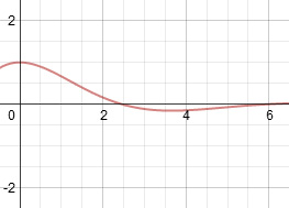
Let's take a look at the resulting motion from simulating position over time.
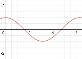 |
We start without any velocity but are not at equilibrium so we start to move towards it and then oscillate forever |
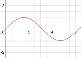 |
We start at equilibrium, but have an initial velocity so we move away and then oscillate forever. |
 |
We are already at equilibrium so we stay there. |
As we can see from these examples, simple harmonic motion alone is not suitable for a game camera. The camera needs to settle at equilibrium rather than shooting past it and oscillating forever. It's velocity needs to dampen over time which brings us to the problem of damped harmonic motion
Damped Simple Harmonic Motion
A damped spring is just like our simple spring with an additional force. In the simple spring case, we had a force proportional to our distance from the equilibrium position. This caused us to always accelerate towards equilibrium, but never come to rest at it (except for the trivial case where we started there with no motion). In order to settle at equilibrium, we add a force proportional to our velocity in the case of damped springs.
\(x = p - r\)
\(F = -\beta v - kx\)
Once again, \(p\) is the current position, \(r\) is the equilibrium position, \(k\) is the spring constant and \(v\) is the current velocity. The new variable, \(\beta\), is the viscous damping coefficient. Higher values of \(\beta\) will create a stronger force against the current velocity.
Using Newton's second, we can work towards our ordinary differential equation.
\(F = ma\)
\(F= -kx - \beta v\)
\(ma = -\beta v - kx\)
\(ma + \beta v + kx = 0\)
Rearranging the equation and defining some new variables will simplify our lives in the following math. The \(\omega\) variable is the same angular frequency variable we had in simple harmonic motion. The new variable, \(\zeta\), is our damping ratio which I will discuss later.
\(a + {\beta \over m}v + {k \over m}x = 0\)
\(a + {\beta \over \sqrt m \sqrt m}v + {k \over m}x = 0\)
\(a + 2 {\beta \over 2 \sqrt m \sqrt m }v + {k \over m}x = 0\)
\(a + 2 {\beta \sqrt k \over 2 \sqrt m \sqrt m \sqrt k}v + {k \over m}x = 0\)
\(a + 2 {\sqrt k \over \sqrt m} {\beta \over 2 \sqrt m \sqrt k}v + {k \over m}x = 0\)
\(a + 2 \sqrt{ k \over m} {\beta \over 2 \sqrt{m k} }v + {k \over m}x = 0\)
\(\omega = \sqrt{k \over m}\)
\(\zeta = { \beta \over 2 \sqrt{mk} }\)
\(a + 2 \omega \zeta v + \omega^2 x = 0\)
We now have our homogeneous linear ODE for damped simple harmonic motion.
General Solution
To solve for the general solution of \(x\) we once again follow Euler's lead and let \(x = e^{zt}\) to simplify.
\(x = e^{z t}\)
\(v = {dx \over dt} = ze^{z t}\)
\(a = {dv \over dt} = z^2 e^{z t}\)
\(a + 2 \omega \zeta v + \omega^2 x = 0\)
\(z^2 e^{z t} + 2 \omega \zeta z e^{zt} + \omega^2 e^{z t} = 0\)
\((z^2 + 2 \omega \zeta z + \omega^2) e^{z t} = 0\)
Dividing both sides by \(e ^ {z t}\) gives us the characteristic equation:
\(z^2 + 2 \omega \zeta z + \omega^2 = 0\)
In order to solve for \(z\), we need to use the quadratic formula which states that the roots of an equation in the form \(Az^2+Bz+C=0\) are given by
\(z=\frac{-B \pm \sqrt {B^2-4AC}}{2 A }\)
Plugging in our coefficients we get
\(A = 1\)
\(B = 2 \omega \zeta\)
\(C = \omega^2\)
\(z=\frac{-2 \omega \zeta \pm \sqrt {(2 \omega \zeta)^2-4 \omega^2}}{2}\)
\(z=\frac{-2 \omega \zeta \pm \sqrt {4 \omega^2 \zeta^2-4 \omega^2}}{2}\)
\(z=\frac{-2 \omega \zeta \pm \sqrt {4 \omega^2 (\zeta^2-1)}}{2}\)
\(z=\frac{-2 \omega \zeta \pm 2 \omega \sqrt {\zeta^2-1}}{2}\)
\(z=-\omega \zeta \pm \omega \sqrt {\zeta^2-1}\)
This gives us two solutions
\(z_1=-\omega \zeta - \omega \sqrt {\zeta^2-1}\)
\(z_2=-\omega \zeta + \omega \sqrt {\zeta^2-1}\)
Both of these equations have a square root with a \(\zeta\) inside it. \(\zeta\) represents the damping ratio and defines how our motion decays over time. Depending on the value of \(\zeta\), we will end up with two real roots, one real root or two complex roots. These correspond to over-damped, critically damped and under-damped harmonic motion respectively. We will solve each one in turn.
Over-damped Simple Harmonic Motion
For over-damped motion, \(\zeta \; > \; 1\). An over-damped spring will never oscillate, but reaches equilibrium at a slower rate than a critically damped spring.
Because \(\zeta > 1\), we know that \(z_1\) and \(z_2\) will be real numbers. Rather than expanding them back out, let's continue to use those variables in our two linearly independent solutions.
\(x_1 = e^{z_1 t}\)
\(x_2 = e^{z_2 t}\)
We can now build our general solution to the linear ODE as a liner combination of our independent solutions by adding the scalar constants \(c_1\) and \(c_2\).
\(x(t) = c_1 x_1 + c_2 x_2\)
\(x(t) = c_1 e^{z_1 t} + c_2 e^{z_2 t}\)
Taking the derivative gives us the general solution for velocity.
\(v(t) = c_1 z_1 e^{z_1 t} + c_2 z_2 e^{z_2 t}\)
In order to get the desired particular solution, we can solve for the constants based on our initial state.
First, we solve \(x(t)\) for a time value of \(t=0\).
\(x(0) = c_1 e^{z_1 0} + c_2 e^{z_2 0}\)
\(x(0) = c_1 + c_2\)
Next, we solve \(v(t)\) for a time value of \(t=0\).
\(v(0) = c_1 z_1 e^{z_1 0} + c_2 z_2 e^{z_2 0}\)
\(v(0) = c_1 z_1 + c_2 z_2\)
Based on the \(x(0)\) and \(v(0)\) equations, we can solve for \(c_1\) and \(c_2\). Let's also let \(x_0 = x(0)\) and \(v_0 = v(0)\) to simplify the equations a bit.
\(c_2 = x_0 - c_1\)
\(v_0 = c_1 z_1 + (x_0 - c_1) z_2\)
\(v_0 = c_1 z_1 + x_0 z_2 - c_1 z_2\)
\(v_0 = x_0 z_2 + c_1 (z_1 - z_2)\)
\(c_1 = {v_0 - x_0 z_2 \over z_1 - z_2}\)
\(c_2 = x_0 - {v_0 - x_0 z_2 \over z_1 - z_2}\)
Now substitute the values for \(c_1\) and \(c_2\) back into the equation for \(x(t)\).
\(x(t) = {v_0 - x_0 z_2 \over z_1 - z_2} e^{z_1 t} \; + \; (x_0 - {v_0 - x_0 z_2 \over z_1 - z_2}) e^{z_2 t}\)
Next we do the same for\(v(t)\).
\(v(t) = {v_0 - x_0 z_2 \over z_1 - z_2} z_1 e^{z_1 t} \; + \; (x_0 - {v_0 - x_0 z_2 \over z_1 - z_2}) z_2 e^{z_2 t}\)
These equations let us calculate a new position and velocity for an over-damped spring based on an elapsed time from an initial position and velocity.
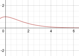
Let's take a look at the resulting motion from simulating position over time.
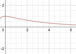 |
We start without any velocity but are not at equilibrium so we start to move towards it. Due to being over-damped, it takes us a long time to reach equilibrium. |
 |
We start with velocity moving away from equilibrium, but our motion quickly dampens out. Due to being over-damped, it takes us a long time to reach equilibrium. |
Critically Damped Harmonic Motion
For critically damped motion, \(\zeta = 1\). A critically damped spring will reach equilibrium as fast as possible without oscillating.
Let's solve for \(z_1\) and \(z_2\).
\(z_1 = -\omega \zeta - \omega \sqrt {\zeta^2-1} = -\omega 1 - \omega \sqrt {1-1} = -\omega\)
\(z_2 = -\omega \zeta + \omega \sqrt {\zeta^2-1} = -\omega 1 + \omega \sqrt {1-1} = -\omega\)
We have a problem here because \(z_1\) and \(z_2\) are both equal to the same value. These are called repeated roots of the characteristic equation. If we were to substitute \(z_1\) and \(z_2\) back into our original equations for \(x_1\) and \(x_2\), we would get
\(x_1 = e^{z_1 t} = e^{-\omega t}\)
\(x_2 = e^{z_2 t} = e^{-\omega t}\)
This is normally where we would combine \(x_1\) and \(x_2\) into a general solution, but that won't work here because they are not linearly independent solutions. They are the same solution. I said previously that a second degree linear ODE must have two linearly independent solutions and that still stands. If you were to follow the math along from here under the assumption that we only have one solution, you would eventually hit a wall where your equations became nonsensical.
\(x(t) = f(t) x_1 = f(t) e^{-\omega t}\)
Now we will try to solve for \(f(t)\) by solving the velocity and acceleration derivatives of \(x(t)\). To do this, we need to use the product rule. Let \(f^\prime(t)\) and \(f^{\prime \prime}(t)\) be the first and second derivatives of \(f(t)\) respectively.
\(v(t) = {d \over dt}x(t)\)
\(v(t) = f^\prime(t) e^{-\omega t} - f(t) \omega e^{-\omega t}\)
\(a(t) = {d \over dt}v(t)\)
\(a(t) = f^{\prime \prime}(t) e^{-\omega t} - f^{\prime}(t) \omega e^{-\omega t} - f^{\prime}(t) \omega e^{-\omega t} + f(t) \omega^2 e^{-\omega t}\)
\(a(t) = f^{\prime \prime}(t) e^{-\omega t} - 2 f^{\prime}(t) \omega e^{-\omega t} + f(t) \omega^2 e^{-\omega t}\)
Simplify by factoring out \(e^{-\omega t}\).
\(v(t) = e^{-\omega t} \Big(f^\prime(t) - f(t) \omega \Big)\)
\(a(t) = e^{-\omega t} \Big(f^{\prime \prime}(t) -2 f^{\prime}(t) \omega + f(t) \omega^2 \Big)\)
Now substitute back into our original equation of \(a + 2 \omega \zeta v + \omega^2 x = 0\) and simplify
\(a(t) + 2 \omega \zeta v(t) + \omega^2 x(t) = 0\)
\(e^{-\omega t} \Big(f^{\prime \prime}(t) -2 f^{\prime}(t) \omega + f(t) \omega^2 \Big) \; + \; 2 \omega \zeta e^{-\omega t} \Big(f^\prime(t) - f(t) \omega \Big) \; + \; \omega^2 f(t) e^{-\omega t} = 0\)
\(e^{-\omega t} \Big(f^{\prime \prime}(t) \; - \; 2 f^{\prime}(t) \omega \; + \; f(t) \omega^2 \; + \; 2 \omega \zeta f^\prime(t) \; - \; 2 \omega^2 \zeta f(t) \; + \; \omega^2 f(t) \Big) = 0\)
\(e^{-\omega t} \Big(f^{\prime \prime}(t) \; - \; 2 f^{\prime}(t) \omega \; + \; 2 f(t) \omega^2 \; + \; 2 \omega \zeta f^\prime(t) \; - \; 2 \omega^2 \zeta f(t) \Big) = 0\)
\(e^{-\omega t} \Big(f^{\prime \prime}(t) \; + \; 2 f^{\prime}(t) \omega(\zeta - 1) \; + \; 2 f(t) \omega^2 \; - \; 2 \omega^2 \zeta f(t) \Big) = 0\)
\(e^{-\omega t} \Big(f^{\prime \prime}(t) \; + \; 2 f^{\prime}(t) \omega(\zeta - 1) \; + \; 2 f(t) \omega^2 ( 1 - \zeta) \Big) = 0\)
Because we are in the critically damped case, we know \(\zeta = 1\) and can simplify further.
\(e^{-\omega t} \Big(f^{\prime \prime}(t) \; + \; 2 f^{\prime}(t) \omega(1 - 1) \; + \; 2 f(t) \omega^2 ( 1 - 1) \Big) = 0\)
\(e^{-\omega t} f^{\prime \prime}(t) = 0\)
The first term, \(e^{-\omega t}\), will never be zero regardless of the values for \(\omega\) and \(t\). Thus we can divide it out of the equation to get:
\(f^{\prime \prime}(t) = 0\)
So we know our functions second derivative is zero, but what we really want to know is the function itself. So, let's integrate back up.
\(f^{\prime \prime}(t) = 0\)
\(f^{\prime}(t) = c_1\)
\(f(t) = c_1 t \; + \; c_2\)
Now, let's plug our solution for \(f(x)\) back into our guess at the general solution to the system.
\(x(t) = f(t) e^{-\omega t}\)
\(x(t) = (c_1 t + c_2) e^{-\omega t}\)
As expected, we have found a general solution that is the sum of two linearly independent solutions scaled by arbitrary constants.
Taking the derivative gives us the general solution for velocity.
\(v(t) = c_1 e^{-\omega t} - (c_1 t + c_2) \omega e^{-\omega t}\)
\(v(t) = \Big(c_1 - (c_1 t + c_2) \omega \Big) e^{-\omega t}\)
\(v(t) = \Big( c_1(1 - \omega t) - c_2 \omega \Big) e^{-\omega t}\)
In order to get the desired particular solution, we can solve for the constants based on our initial state.
First, we solve \(x(t)\) for a time value of \(t=0\).
\(x(0) = (c_1 0 + c_2) e^{-\omega 0}\)
\(x(0) = c_2\)
Next, we solve \(v(t)\) for a time value of \(t=0\).
\(v(0) = \Big( c_1(1 - \omega 0) - c_2 \omega \Big) e^{-\omega 0}\)
\(v(0) = c_1 - c_2 \omega\)
Based on the \(x(0)\) and \(v(0)\) equations, we can solve for \(c_1\) and \(c_2\). Let's also let \(x_0 = x(0)\) and \(v_0 = v(0)\) to simplify the equations a bit.
\(c_2 = x_0\)
\(v_0 = c_1 - x_0 \omega\)
\(c_1 = v_0 + x_0 \omega\)
Now substitute the values for \(c_1\) and \(c_2\) back into the equation for \(x(t)\).
\(x(t) = \Big( (v_0 + x_0 \omega) t + x_0 \Big) e^{-\omega t}\)
Next we do the same for \(v(t)\).
\(v(t) = \Big( (v_0 + x_0 \omega)(1 - \omega t) - x_0 \omega \Big) e^{-\omega t}\)
\(v(t) = \Big( v_0 + x_0 \omega - v_0 \omega t - x_0 \omega^2 t - x_0 \omega \Big) e^{-\omega t}\)
\(v(t) = \Big( v_0 - (v_0 + x_0 \omega) \omega t \Big) e^{-\omega t}\)
These equations let us calculate a new position and velocity for a critically damped spring based on an elapsed time from an initial position and velocity.
Let's take a look at the resulting motion from simulating position over time.
 |
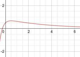
We start without any velocity but are not at equilibrium so we start to move towards it. Due to being critically-damped, our position and velocity reach equilibrium as soon as possible for our given angular frequency. |
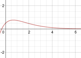 |
We start with velocity moving away from equilibrium, but our motion quickly dampens out. Due to being critically-damped, our position and velocity reach equilibrium as soon as possible for our given angular frequency. |
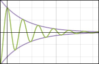
Under-damped Simple Harmonic Motion
For under-damped motion, \(0 \; \le \; \zeta \; < \; 1\). An under-damped spring will reach equilibrium the fastest, but also overshoots it and continues to oscillate as its amplitude decays over time.
Because \(\zeta \; < \; 1\), we know that \(\sqrt{\zeta^2 - 1}\) is a complex number. By rearranging, we can expose the imaginary term as follows.
\(\sqrt{\zeta^2 - 1} = \sqrt{-1 * -(\zeta^2 - 1)} = \sqrt{-1} \sqrt{-(\zeta^2 - 1)} = i \sqrt{1 - \zeta^2}\)
Using this equality, we can update our roots.
\(z=-\omega \zeta \pm \omega i \sqrt{1 - \zeta^2)}\)
Before continuing, let's make our equations a bit less verbose by defining a new variable, \(\alpha\).
\(\alpha = \omega \sqrt{1 - \zeta^2}\)
\(z=-\omega \zeta \pm i \alpha\)
Plugging back into our equation for \(x\), we get:
\(x = e^{z t}\)
\(x = e^{(-\omega \zeta \pm i \alpha) t}\)
Breaking up the \(\pm\) into our two solutions, we have:
\(x_1 = e^{-\omega \zeta t + i \alpha t}\)
\(x_2 = e^{-\omega \zeta t - i \alpha t}\)
If we split the exponent, we can apply Euler's formula.
\(x_1 = e^{-\omega \zeta t} e^{i \alpha t}\)
\(x_1 = e^{-\omega \zeta t} \Big( \cos(\alpha t) + i \sin(\alpha t) \Big)\)
\(x_2 = e^{-\omega \zeta t} e^{-i\alpha t}\)
\(x_2 = e^{-\omega \zeta t} \Big( \cos(-\alpha t) + i \sin(-\alpha t) \Big)\)
Using the trig identities \(\cos(-\theta)=\cos(\theta)\) and \(\sin(-\theta)=-\sin(\theta)\), we can simplify \(x_2\).
\(x_2 = e^{-\omega \zeta t} \Big( \cos(\alpha t) - i \sin(\alpha t) \Big)\)
We now have two linearly independent solutions to the ODE, but they still contain imaginary terms. We are only interested in real solutions so it would be preferable to remove the imaginary parts sooner than later. To do this we will generate two new basis equations as linear sums of our existing equations. We will choose scaling constants that cancel out the imaginary while still getting linearly independent results, \(x_3\) and \(x_4\).
\(x_3 = {1 \over 2} x_1 + {1 \over 2} x_2\)
\(x_3 = {1 \over 2} e^{-\omega \zeta t} \Big( \cos(\alpha t) + i \sin(\alpha t) \Big) + {1 \over 2} e^{-\omega \zeta t} \Big( \cos(\alpha t) - i \sin(\alpha t) \Big)\)
\(x_3 = {1 \over 2} e^{-\omega \zeta t} \Big( \cos(\alpha t) + i \sin(\alpha t) + \cos(\alpha t) - i \sin(\alpha t) \Big)\)
\(x_3 = e^{-\omega \zeta t} \cos(\alpha t)\)
\(x_4 = {1 \over {2 i}} x_1 - {1 \over {2 i}} x_2\)
\(x_4 = {1 \over {2 i}} e^{-\omega \zeta t} \Big( \cos(\alpha t) + i \sin(\alpha t) \Big) - {1 \over {2 i}} e^{-\omega \zeta t} \Big( \cos(\alpha t) - i \sin(\alpha t) \Big)\)
\(x_4 = {1 \over {2 i}} e^{-\omega \zeta t} \Big( \cos(\alpha t) + i \sin(\alpha t) - \cos(\alpha t) + i \sin(\alpha t) \Big)\)
\(x_4 = e^{-\omega \zeta t} \sin(\alpha t)\)
We can now build our general solution to the linear ODE as a liner combination of our independent solutions by adding the scalar constants \(c_1\) and \(c_2\).
\(x(t) = c_1 x_3 + c_2 x_4\)
\(x(t) = c_1 e^{-\omega \zeta t} \cos(\alpha t) + c_2 e^{-\omega \zeta t} \sin(\alpha t)\)
\(x(t) = e^{-\omega \zeta t} \Big( c_1 \cos(\alpha t) + c_2 \sin(\alpha t) \Big)\)
Taking the derivative gives us the general solution for velocity.
\(v(t) = -\omega \zeta e^{-\omega \zeta t} \Big( c_1 \cos(\alpha t) + c_2 \sin(\alpha t) \Big) + e^{-\omega \zeta t} \Big( -c_1 \alpha \sin(\alpha t) + c_2 \alpha \cos(\alpha t) \Big)\)
\(v(t) = -e^{-\omega \zeta t} \Big( \omega \zeta c_1 \cos(\alpha t) + \omega \zeta c_2 \sin(\alpha t) + c_1 \alpha \sin(\alpha t) - c_2 \alpha \cos(\alpha t) \Big)\)
\(v(t) = -e^{-\omega \zeta t} \Big( (c_1 \omega \zeta - c_2 \alpha) \cos(\alpha t) + ( c_1 \alpha + c_2 \omega \zeta) \sin(\alpha t) \Big)\)
In order to get the desired particular solution, we can solve for the constants based on our initial state.
First, we solve \(x(t)\) for a time value of \(t=0\).
\(x(0) = e^{-\omega \zeta 0} \Big( c_1 \cos(\alpha 0) + c_2 \sin(\alpha 0) \Big)\)
\(x(0) = c_1\)
Next, we solve \(v(t)\) for a time value of \(t=0\).
\(v(0) = -e^{-\omega \zeta 0} \Big( (c_1 \omega \zeta - c_2 \alpha) \cos(\alpha 0) + ( c_1 \alpha + c_2 \omega \zeta) \sin(\alpha 0) \Big)\)
\(v(0) = -(c_1 \omega \zeta - c_2 \alpha)\)
\(v(0) = -c_1 \omega \zeta + c_2 \alpha\)
Based on the \(x(0)\) and \(v(0)\) equations, we can solve for \(c_1\) and \(c_2\). Let's also let \(x_0 = x(0)\) and \(v_0 = v(0)\) to simplify the equations a bit.
\(c_1 = x_0\)
\(v_0 = -x_0 \omega \zeta + c_2 \alpha\)
\(c_2 = { v_0 + \omega \zeta x_0 \over \alpha}\)
Now substitute the values for \(c_1\) and \(c_2\) back into the equation for \(x(t)\).
\(x(t) = e^{-\omega \zeta t} \Big( x_0 \cos(\alpha t) \; + \; { v_0 + \omega \zeta x_0 \over \alpha} \sin(\alpha t) \Big)\)
Next we do the same for\(v(t)\).
\(v(t) = -e^{-\omega \zeta t} \Big( (x_0 \omega \zeta \; - \; { v_0 + \omega \zeta x_0 \over \alpha} \alpha) \cos(\alpha t) \; + \; (x_0 \alpha \; + \; { v_0 + \omega \zeta x_0 \over \alpha} \omega \zeta) \sin(\alpha t) \Big)\)
These equations let us calculate a new position and velocity for an under-damped spring based on an elapsed time from an initial position and velocity.
Let's take a look at the resulting motion from simulating position over time.
 |
We start without any velocity but are not at equilibrium so we start to move towards it. Due to being under-damped, we continue to overshoot equilibrium with each oscillation, but we overshoot it less and less each time. |
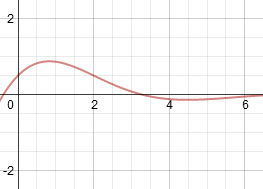 |
We start with velocity moving away from equilibrium, but our motion quickly dampens out. Due to being under-damped, we continue to overshoot equilibrium with each oscillation, but we overshoot it less and less each time. |
Writing the Code
We can now program a damped simple harmonic oscillator. Because simulating damped springs requires calls to potentially expensive trigonometric and exponential functions, I've split the process into two steps. The first computes a set of coefficients for the position and velocity parameters by expanding the relevant equations. These coefficients can then be used to quickly update multiple springs using the same angular frequency, damping ratio and time step. If your simulation updates at a locked time step, you can even cache off the coefficients once at initialization time and use them every frame!
These code samples are released under the following license.
/******************************************************************************
  Copyright (c) 2008-2012 Ryan Juckett
  http://www.ryanjuckett.com/

  This software is provided 'as-is', without any express or implied
  warranty. In no event will the authors be held liable for any damages
  arising from the use of this software.

  Permission is granted to anyone to use this software for any purpose,
  including commercial applications, and to alter it and redistribute it
  freely, subject to the following restrictions:

  1. The origin of this software must not be misrepresented; you must not
     claim that you wrote the original software. If you use this software
     in a product, an acknowledgment in the product documentation would be
     appreciated but is not required.

  2. Altered source versions must be plainly marked as such, and must not be
     misrepresented as being the original software.

  3. This notice may not be removed or altered from any source
     distribution.
******************************************************************************/
Call the CalcDampedSpringMotionParams function once with your parameters to initialize a tDampedSpringMotionParams structure. Then call UpdateDampedSpringMotion with pointers referencing the position and velocity values for each spring that needs updating.
//******************************************************************************
// Cached set of motion parameters that can be used to efficiently update
// multiple springs using the same time step, angular frequency and damping
// ratio.
//******************************************************************************
struct tDampedSpringMotionParams
{
	// newPos = posPosCoef*oldPos + posVelCoef*oldVel
	float m_posPosCoef, m_posVelCoef;
	// newVel = velPosCoef*oldPos + velVelCoef*oldVel
	float m_velPosCoef, m_velVelCoef;
};

//******************************************************************************
// This function will compute the parameters needed to simulate a damped spring
// over a given period of time.
// - An angular frequency is given to control how fast the spring oscillates.
// - A damping ratio is given to control how fast the motion decays.
//     damping ratio > 1: over damped
//     damping ratio = 1: critically damped
//     damping ratio < 1: under damped
//******************************************************************************
void CalcDampedSpringMotionParams(
	tDampedSpringMotionParams* pOutParams,       // motion parameters result
	float	                   deltaTime,        // time step to advance
	float	                   angularFrequency, // angular frequency of motion
	float	                   dampingRatio)     // damping ratio of motion
{
	const float epsilon = 0.0001f;

	// force values into legal range
	if (dampingRatio     < 0.0f) dampingRatio     = 0.0f;
	if (angularFrequency < 0.0f) angularFrequency = 0.0f;

	// if there is no angular frequency, the spring will not move and we can
	// return identity
	if ( angularFrequency < epsilon )
	{
		pOutParams->m_posPosCoef = 1.0f; pOutParams->m_posVelCoef = 0.0f;
		pOutParams->m_velPosCoef = 0.0f; pOutParams->m_velVelCoef = 1.0f;
		return;
	}

	if (dampingRatio > 1.0f + epsilon)
	{
		// over-damped
		float za = -angularFrequency * dampingRatio;
		float zb = angularFrequency * sqrtf(dampingRatio*dampingRatio - 1.0f);
		float z1 = za - zb;
		float z2 = za + zb;

		float e1 = expf( z1 * deltaTime );
		float e2 = expf( z2 * deltaTime );

		float invTwoZb = 1.0f / (2.0f*zb); // = 1 / (z2 - z1)

		float e1_Over_TwoZb = e1*invTwoZb;
		float e2_Over_TwoZb = e2*invTwoZb;

		float z1e1_Over_TwoZb = z1*e1_Over_TwoZb;
		float z2e2_Over_TwoZb = z2*e2_Over_TwoZb;

		pOutParams->m_posPosCoef =  e1_Over_TwoZb*z2 - z2e2_Over_TwoZb + e2;
		pOutParams->m_posVelCoef = -e1_Over_TwoZb    + e2_Over_TwoZb;

		pOutParams->m_velPosCoef = (z1e1_Over_TwoZb - z2e2_Over_TwoZb + e2)*z2;
		pOutParams->m_velVelCoef = -z1e1_Over_TwoZb + z2e2_Over_TwoZb;
	}
	else if (dampingRatio < 1.0f - epsilon)
	{
		// under-damped
		float omegaZeta = angularFrequency * dampingRatio;
		float alpha     = angularFrequency * sqrtf(1.0f - dampingRatio*dampingRatio);

		float expTerm = expf( -omegaZeta * deltaTime );
		float cosTerm = cosf( alpha * deltaTime );
		float sinTerm = sinf( alpha * deltaTime );

		float invAlpha = 1.0f / alpha;

		float expSin = expTerm*sinTerm;
		float expCos = expTerm*cosTerm;
		float expOmegaZetaSin_Over_Alpha = expTerm*omegaZeta*sinTerm*invAlpha;

		pOutParams->m_posPosCoef = expCos + expOmegaZetaSin_Over_Alpha;
		pOutParams->m_posVelCoef = expSin*invAlpha;

		pOutParams->m_velPosCoef = -expSin*alpha - omegaZeta*expOmegaZetaSin_Over_Alpha;
		pOutParams->m_velVelCoef =  expCos - expOmegaZetaSin_Over_Alpha;
	}
	else
	{
		// critically damped
		float expTerm     = expf( -angularFrequency*deltaTime );
		float timeExp     = deltaTime*expTerm;
		float timeExpFreq = timeExp*angularFrequency;

		pOutParams->m_posPosCoef = timeExpFreq + expTerm;
		pOutParams->m_posVelCoef = timeExp;

		pOutParams->m_velPosCoef = -angularFrequency*timeExpFreq;
		pOutParams->m_velVelCoef = -timeExpFreq + expTerm;
	}
}

//******************************************************************************
// This function will update the supplied position and velocity values over
// according to the motion parameters.
//******************************************************************************
void UpdateDampedSpringMotion(
	float*                           pPos,           // position value to update
	float*                           pVel,           // velocity value to update
	const float                      equilibriumPos, // position to approach
	const tDampedSpringMotionParams& params)         // motion parameters to use
{
	const float oldPos = *pPos - equilibriumPos; // update in equilibrium relative space
	const float oldVel = *pVel;

	(*pPos) = oldPos*params.m_posPosCoef + oldVel*params.m_posVelCoef + equilibriumPos;
	(*pVel) = oldPos*params.m_velPosCoef + oldVel*params.m_velVelCoef;
}
Comments