
Biarc Interpolation
Why would you want a circular interpolation? One reason might be that it is pleasing to eye, but it also has some practical use. If you are making a level editing tool that places roads (or making a game with procedural roads), you will may want turns to resemble their real-world counterparts. A second example, and the one I most often run across, is generating trails behind swords. Sword swings are often animated very fast. You only get a few sample points as the sword arcs through the attack. If you play the animation in slow motion, you'll find that the tip of the sword takes a rather circular path. By generating circular arcs between the sample points, a clean trail can be generated.
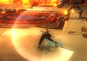
Here's an example of the sword trails I programmed for Spyborgs. There might have been only five or six samples along the whole spin, but I was able to create a smooth arc of vertices. The Spyborgs algorithm was a bit different from what I'm going to present here, but generated similar results (they were actually slightly worse if you know what to look for).
So, how are we going to create these curves? The solution lies in a piece of geometry called a biarc.
Biarcs
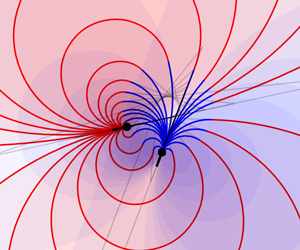
A biarc is a curve composed of two circular arcs such that they connect with a matching tangent. Almost every pair of control points can be connected by a biarc and the ones that fail don't really come up in practice. Here are some example biarcs connecting a red control point to a blue control point.
Once you can solve for a biarc between two control points, it is trivial to connect a sequence of control points with a chain of biarcs. This is known as a piecewise circular curve.
The Goal
We are going to take two control points as an input and generate two circular arcs as an output.
The input tangents are assumed to be normalized. In other words:
\( \lvert t_1 \rvert = 1 \)
\( \lvert t_2 \rvert = 1 \)
Finding the Connection
Before we can solve for the arcs, we need to find the connection point, \(p_m\).
We can define points \(q_1\) and \(q_2\) at the intersections of the line extending from the connection point along the connection tangent with the lines extending from the control points along the control tangents. Let the distances \(\lvert q_1 - p_1\rvert\) and \(\lvert q_1 - p_m\rvert\) be \(d_1\) and the distances \(\lvert q_2 - p_2\rvert\) and \(\lvert q_2 - p_m\rvert\) be \(d_2\). We can now define the following equations:
\( q_1 = p_1 + d_1 t_1 \)
\( q_2 = p_2 - d_2 t_2 \)
\( \lvert q_2 - q_1 \rvert = d_1 + d_2 \)
Next, solve for the connection point as weighted blend of the two corner points.
\( p_m = q_1 * \frac{d_2}{d_1 + d_2} + q_2 * \frac{d_1}{d_1 + d_2} \)
\( p_m = (p_1 + d_1 t_1) * \frac{d_2}{d_1 + d_2} + (p_2 - d_2 t_2) * \frac{d_1}{d_1 + d_2} \)
To simplify future math, let's also define the following vector:
\( v = p_2 - p_1 \)
Solve for \(d_2\) in terms of \(d_1\) by squaring the corner point distance equality and substituting in the equations for \(q_1\) and \(q_2\).
\( (q_2 - q_1) \cdot (q_2 - q_1) = (d_1 + d_2)^2 \)
\( (p_2 - d_2 t_2 - p_1 - d_1 t_1) \cdot (p_2 - d_2 t_2 - p_1 - d_1 t_1) = (d_1 + d_2)^2 \)
\( (v - d_2 t_2 - d_1 t_1) \cdot (v - d_2 t_2 - d_1 t_1) = d_1^2 + 2 d_1 d_2 + d_2^2 \)
\( v \cdot v - 2 d_2 v \cdot t_2 - 2 d_1 v \cdot t_1 + d_2^2 t_2 \cdot t_2 + 2 d_1 d_2 t_1 \cdot t_2 + d_1^2 t_1 \cdot t_1 = d_1^2 + 2 d_1 d_2 + d_2^2 \)
\( v \cdot v - 2 d_2 v \cdot t_2 - 2 d_1 v \cdot t_1 + d_2^2 + 2 d_1 d_2 t_1 \cdot t_2 + d_1^2 = d_1^2 + 2 d_1 d_2 + d_2^2 \)
\( v \cdot v - 2 d_2 v \cdot t_2 - 2 d_1 v \cdot t_1 + 2 d_1 d_2 (t_1 \cdot t_2 - 1) = 0\)
\( v \cdot v - 2 d_1 v \cdot t_1 - d_2 (2 v \cdot t_2 - 2 d_1 (t_1 \cdot t_2 - 1)) = 0\)
\( d_2 = \frac {v \cdot v - 2 d_1 v \cdot t_1} { 2 v \cdot t_2 - 2 d_1 (t_1 \cdot t_2 - 1) }\)
\( d_2 = \frac { \frac {1}{2} v \cdot v - d_1 v \cdot t_1} { v \cdot t_2 - d_1 (t_1 \cdot t_2 - 1) }\)
Edge Cases
Finding the Center
With the connection point found, we can solve for the circle centers. Let's define a vector, \(n_1\), perpendicular to \(t_1\). This ends up being a normalized vector that it is parallel to \((c_1 - p_1)\). Note that the direction could point from \(c_1\) to \(p_1\) or from \(p_1\) to \(c_1\).
\( t_1 = \begin{bmatrix}t_{1x}\\t_{1y}\end{bmatrix} \)
\( n_1 = \begin{bmatrix}-t_{1y}\\t_{1x}\end{bmatrix} \)
We can now define \(c_1\) as a point somewhere along vector \(n_1\) that is equidistant from \(p_1\) and \(p_m\).
\( c_1 = p_1 + s_1 n_1 \)
\( \lvert p_1 - c_1 \lvert = \lvert p_m - c_1 \lvert \)
Square the equality and simplify.
\( (p_1 - c_1) \cdot (p_1 - c_1) = (p_m - c_1) \cdot (p_m - c_1) \)
\( p_1 \cdot p_1 - 2 p_1 \cdot c_1 + c_1 \cdot c_1 = p_m \cdot p_m - 2 p_m \cdot c_1 + c_1 \cdot c_1 \)
\( 2 p_m \cdot c_1 - 2 p_1 \cdot c_1 = p_m \cdot p_m - p_1 \cdot p_1 \)
\( 2 c_1 \cdot (p_m - p_1) = p_m \cdot p_m - p_1 \cdot p_1 \)
Substitute in for \(c_1\) and solve for \(s_1\).
\( 2 (p_1 + s_1 n_1) \cdot (p_m - p_1) = p_m \cdot p_m - p_1 \cdot p_1 \)
\( 2 (p_1 \cdot p_m - p_1 \cdot p_1 + s_1 n_1 \cdot p_m - s n_1 \cdot p_1) = p_m \cdot p_m - p_1 \cdot p_1 \)
\( 2s_1 (n_1 \cdot p_m - n_1 \cdot p_1) = p_m \cdot p_m - p_1 \cdot p_1 - 2 (p_1 \cdot p_m - p_1 \cdot p_1)\)
\( 2s_1 n_1 \cdot (p_m - p_1) = p_m \cdot p_m - 2 p_1 \cdot p_m + p_1 \cdot p_1\)
\( 2s_1 n_1 \cdot (p_m - p_1) = (p_m - p_1) \cdot (p_m - p_1)\)
\( s_1 = \frac {(p_m - p_1) \cdot (p_m - p_1)}{ 2 n_1 \cdot (p_m - p_1) } \)
Putting it all together we have our solution for \(c_1\).
\( c_1 = p_1 + \frac {(p_m - p_1) \cdot (p_m - p_1)}{ 2 n_1 \cdot (p_m - p_1) } n_1 \)
By inspecting the denominator in the above equation, we can see that it will be zero if the vector from \(p_1\) to \(p_m\) is collinear with \(t_1\). The center of the circle essentially gets pushed out to infinity which leaves us with a straight line between \(p_1\) and \(p_m\) instead of an arc.
Using the same method for \(c_2\) gives:
\( t_2 = \begin{bmatrix}t_{2x}\\t_{2y}\end{bmatrix} \)
\( n_2 = \begin{bmatrix}-t_{2y}\\t_{2x}\end{bmatrix} \)
\( s_2 = \frac {(p_m - p_2) \cdot (p_m - p_2)}{ 2 n_2 \cdot (p_m - p_2) } \)
\( c_2 = p_2 + \frac {(p_m - p_2) \cdot (p_m - p_2)}{ 2 n_2 \cdot (p_m - p_2) } n_2 \)
When we have valid arcs, the radii are:
\( r_1 = \lvert s_1 \rvert \)
\( r_2 = \lvert s_2 \rvert \)
Choosing a Direction
Now we need to choose which direction to rotate about the center points. This depends on the signs of \(d_1\) and \(d_2\). For the positive case, we take the shorter path around the circle. For the negative case, we take the longer path. Let's look at some examples.
The final step is to solve for the angle of rotation. To help with this we are going to define the \( \times \) operator like so.
\( a \times b = a_x b_y - a_y b_x\)
This gives us what would be the z-component of a 3-dimensional cross product. It is equivalent to \(\lvert a \rvert \lvert b \rvert \sin \alpha\) where \(\alpha\) is the angle between vectors \(a\) and \(b\). Due to the \(sin\) value, we can determine the direction of rotation based on a positive or negative result.
If an arc's radius is zero, the angle can be set to zero. Otherwise, it is computed like so:
\(o_{p1} = \frac { p_1 - c_1 } {r_1} \)
\(o_{m1} = \frac { p_m - c_1 } {r_1} \)
\(o_{p2} = \frac { p_2 - c_2 } {r_2} \)
\(o_{m2} = \frac { p_m - c_2 } {r_2} \)
\(\theta_1 = \begin{cases} \arccos(o_{p1} \cdot o_{m1}) & d_1 \gt 0 \text{ and } o_{p1} \times o_{m1} \gt 0 \\ -\arccos(o_{p1} \cdot o_{m1}) & d_1 \gt 0 \text{ and } o_{p1} \times o_{m1} \le 0 \\ -2\pi + \arccos(o_{p1} \cdot o_{m1}) & d_1 \le 0 \text{ and } o_{p1} \times o_{m1} \gt 0 \\ 2\pi - \arccos(o_{p1} \cdot o_{m1}) & d_1 \le 0 \text{ and } o_{p1} \times o_{m1} \le 0 \end{cases}\)
\(\theta_2 = \begin{cases} \arccos(o_{p2} \cdot o_{m2}) & d_2 \gt 0 \text{ and } o_{p2} \times o_{m2} \gt 0 \\ -\arccos(o_{p2} \cdot o_{m2}) & d_2 \gt 0 \text{ and } o_{p2} \times o_{m2} \le 0 \\ -2\pi + \arccos(o_{p2} \cdot o_{m2}) & d_2 \le 0 \text{ and } o_{p2} \times o_{m2} \gt 0 \\ 2\pi - \arccos(o_{p2} \cdot o_{m2}) & d_2 \le 0 \text{ and } o_{p2} \times o_{m2} \le 0 \end{cases}\)
Choosing d1

Often, it is best to automatically choose a \(d_1\) value. The simplest acceptable approach is to pick a value that will make \(d_1 = d_2\). This creates a rather balanced curve and simplifies some of the computations. Let's substitute \(d_1\) with \(d_2\) in the connection point equation and solve it.
\( p_m = (p_1 + d_2 t_1) * \frac{d_2}{d_2 + d_2} + (p_2 - d_2 t_2) * \frac{d_2}{d_2 + d_2} \)
\( p_m = \frac{p_1 + d_2 t_1}{2} + \frac{p_2 - d_2 t_2}{2} \)
\( p_m = \frac{p_1 + d_2 t_1 + p_2 - d_2 t_2}{2} \)
\( p_m = \frac{p_1 + p_2 + d_2 (t_1 - t_2)}{2} \)
We can do the same for the \(d_2\) equation.
\( d_2 = \frac { \frac {1}{2} v \cdot v - d_2 v \cdot t_1} { v \cdot t_2 - d_2 (t_1 \cdot t_2 - 1) }\)
\( (v \cdot t_2 - d_2 (t_1 \cdot t_2 - 1))d_2 = \frac {1}{2} v \cdot v - d_2 v \cdot t_1\)
\( (v \cdot t_2) d_2 + (1 - t_1 \cdot t_2)d_2^2 + v \cdot t_1 d_2 = \frac {1}{2} v \cdot v \)
\( (1 - t_1 \cdot t_2)d_2^2 + (v \cdot t_2 + v \cdot t_1) * d_2 - \frac {1}{2}v \cdot v = 0 \)
Let \(t = t_1 + t_2\)
\( (1 - t_1 \cdot t_2)d_2^2 + (v \cdot t) * d_2 - \frac {1}{2}v \cdot v = 0 \)
Using the quadratic formula, we get:
\(d_2 = {\Large \frac{ -(v \cdot t) \pm \sqrt { (v \cdot t)^2 - 4 (1 - t_1 \cdot t_2)(- \frac {1}{2}v \cdot v) } }{ 2(1 - t_1 \cdot t_2) } }\)
\(d_2 = {\Large \frac{ -(v \cdot t) \pm \sqrt { (v \cdot t)^2 + 2 (1 - t_1 \cdot t_2)(v \cdot v) } }{ 2 (1 - t_1 \cdot t_2) } }\)
Case 1:
When the quadratic formula is computable, one of the solutions is positive and the other is negative. We always want the positive solution because that represents the shorter arc. The denominator is always positive and the discriminant is going to be greater than \((v \cdot t)^2\) so choosing the plus version will give a positive result.
\(d_2 = {\Large \frac{ -(v \cdot t) + \sqrt { (v \cdot t)^2 + 2 (1 - t_1 \cdot t_2)(v \cdot v) } }{ 2 (1 - t_1 \cdot t_2) } }\)
Case 2:
Because the tangents are normalized, all inputs create a discriminant greater than or equal to zero. Thus we don't need to worry about the square root. However, the denominator can evaluate to zero when the tangents are equal. To support this case we can solve for \(d_2\) again by letting \(t_1 = t_2\).
\( d_2 = \frac { \frac {1}{2} v \cdot v - d_2 v \cdot t_2} { v \cdot t_2 - d_2 (t_2 \cdot t_2 - 1) }\)
\( d_2 = \frac { \frac {1}{2} v \cdot v - d_2 v \cdot t_2} { v \cdot t_2 }\)
\( d_2 (v \cdot t_2) = \frac {1}{2} v \cdot v - d_2 v \cdot t_1\)
\( d_2 (v \cdot t_2) + d_2 v \cdot t_1 = \frac {1}{2} v \cdot v \)
\( 2 d_2 v \cdot t_2 = \frac {v \cdot v}{2} \)
\( d_2 = \frac {v \cdot v}{4 v \cdot t_2 } \)
Case 3:
The final edge case we need to handle occurs when the tangents are equal and \(v\) is perpendicular to them. This will create a zero denominator in the solution for case 2 and implies that \(d_1\) and \(d_2\) are at an infinite distance. This can be handled with two semicircles as seen here:

Interactive Demo
Here's an interactive demo written with HTML5. To move the control points, click and drag them. To move the tangents, click and drag the area just outside the control points. By default, the curve keeps \(d_1\) and \(d_2\) equal, but you can also specify a custom \(d_1\) value below.
Point 1
x: y:
angle:
Point 2
x: y:
angle:
Code
So far, we've just discussed the two dimensional case. Let's write some C++ code to solve the three dimensional case. It's pretty similar except that each of the arcs can be aligned on a different plane. This creates some adjustments in finding the rotation direction and the plane normal. After a few cross products, it all works out.
These code samples are released under the following license.
/******************************************************************************
  Copyright (c) 2014 Ryan Juckett
  http://www.ryanjuckett.com/

  This software is provided 'as-is', without any express or implied
  warranty. In no event will the authors be held liable for any damages
  arising from the use of this software.

  Permission is granted to anyone to use this software for any purpose,
  including commercial applications, and to alter it and redistribute it
  freely, subject to the following restrictions:

  1. The origin of this software must not be misrepresented; you must not
     claim that you wrote the original software. If you use this software
     in a product, an acknowledgment in the product documentation would be
     appreciated but is not required.

  2. Altered source versions must be plainly marked as such, and must not be
     misrepresented as being the original software.

  3. This notice may not be removed or altered from any source
     distribution.
******************************************************************************/
Here's our vector type. It's about as basic as vector types come.
//******************************************************************************
//******************************************************************************
struct tVec3
{
    float x;
    float y;
    float z;
};
Now, let's define some math functions to help with common operations (mostly linear algebra).
//******************************************************************************
// Compute the dot product of two vectors.
//******************************************************************************
float Vec_DotProduct(const tVec3& lhs, const tVec3& rhs)
{
    return lhs.x*rhs.x + lhs.y*rhs.y + lhs.z*rhs.z;
}

//******************************************************************************
// Compute the cross product of two vectors.
//******************************************************************************
void Vec_CrossProduct(tVec3* pResult, const tVec3& lhs, const tVec3& rhs)
{
    float x = lhs.y*rhs.z - lhs.z*rhs.y;
    float y = lhs.z*rhs.x - lhs.x*rhs.z;
    float z = lhs.x*rhs.y - lhs.y*rhs.x;

    pResult->x = x;
    pResult->y = y;
    pResult->z = z;
}

//******************************************************************************
// Compute the sum of two vectors.
//******************************************************************************
void Vec_Add(tVec3* pResult, const tVec3& lhs, const tVec3& rhs)
{
    pResult->x = lhs.x + rhs.x;
    pResult->y = lhs.y + rhs.y;
    pResult->z = lhs.z + rhs.z;
}

//******************************************************************************
// Compute the difference of two vectors.
//******************************************************************************
void Vec_Subtract(tVec3* pResult, const tVec3& lhs, const tVec3& rhs)
{
    pResult->x = lhs.x - rhs.x;
    pResult->y = lhs.y - rhs.y;
    pResult->z = lhs.z - rhs.z;
}

//******************************************************************************
// Compute a scaled vector.
//******************************************************************************
void Vec_Scale(tVec3* pResult, const tVec3& lhs, float rhs)
{
    pResult->x = lhs.x*rhs;
    pResult->y = lhs.y*rhs;
    pResult->z = lhs.z*rhs;
}

//******************************************************************************
// Add a vector to a scaled vector.
//******************************************************************************
void Vec_AddScaled(tVec3* pResult, const tVec3& lhs, const tVec3& rhs, float rhsScale)
{
    pResult->x = lhs.x + rhs.x*rhsScale;
    pResult->y = lhs.y + rhs.y*rhsScale;
    pResult->z = lhs.z + rhs.z*rhsScale;
}

//******************************************************************************
// Compute the magnitude of a vector.
//******************************************************************************
float Vec_Magnitude(const tVec3& lhs)
{
    return sqrtf(Vec_DotProduct(lhs,lhs));
}

//******************************************************************************
// Check if the vector length is within epsilon of 1
//******************************************************************************
bool Vec_IsNormalized_Eps(const tVec3& value, float epsilon)
{
    const float sqrMag = Vec_DotProduct(value,value);
    return      sqrMag >= (1.0f - epsilon)*(1.0f - epsilon)
            &&  sqrMag <= (1.0f + epsilon)*(1.0f + epsilon);
}

//******************************************************************************
// Return 1 or -1 based on the sign of a real number.
//******************************************************************************
inline float Sign(float val)
{
    return (val < 0.0f) ? -1.0f : 1.0f;
}
The algorithm is broken up into two parts. First, we provide a function to compute the pair of arcs making up the curve (this basically covers all of the fun math I showed above). Second, we provide a function to interpolate across the biarc curve. This is the helper type representing a computed arc. It is the output of the first part (biarc computation) and the input to the second part (biarc interpolation).
The set of data stored in this type has been chosen to reduce the number of operations in the interpolation process. This lets the user compute the biarc once, and then compute a bunch of points along it very fast. In our interpolation function, we will do a proper blend across each circular arc, but you might instead want to convert the biarc into something like an approximate Bézier curve such that it is compatible with other systems. In that case, you might not need all these values.
//******************************************************************************
// Information about an arc used in biarc interpolation. Use
// Vec_BiarcInterp_ComputeArcs to compute the values and use Vec_BiarcInterp
// to interpolate along the arc pair.
//******************************************************************************
struct tBiarcInterp_Arc
{
    tVec3   m_center;   // center of the circle (or line)
    tVec3   m_axis1;    // vector from center to the end point
    tVec3   m_axis2;    // vector from center edge perpendicular to axis1
    float   m_radius;   // radius of the circle (zero for lines)
    float   m_angle;    // angle to rotate from axis1 towards axis2
    float   m_arcLen;   // distance along the arc
};
This is a helper function for computing data about a single arc. This isn't intended as a user facing function.
//******************************************************************************
// Compute a single arc based on an end point and the vector from the endpoint
// to connection point.
//******************************************************************************
void BiarcInterp_ComputeArc(
tVec3* pCenter, // Out: Center of the circle or straight line.
float* pRadius, // Out: Zero for straight lines
float* pAngle, // Out: Angle of the arc
const tVec3& point,
const tVec3& tangent,
const tVec3& pointToMid)
{
// assume that the tangent is normalized
assert( Vec_IsNormalized_Eps(tangent,0.01f) );
const float c_Epsilon = 0.0001f;
// compute the normal to the arc plane
tVec3 normal;
Vec_CrossProduct(&normal, pointToMid, tangent);
// Compute an axis within the arc plane that is perpendicular to the
// tangent. This will be coliniear with the vector from the center to
// the end point.
tVec3 perpAxis;
Vec_CrossProduct(&perpAxis, tangent, normal);
const float denominator = 2.0f * Vec_DotProduct(perpAxis, pointToMid);
if (fabs(denominator) < c_Epsilon)
{
// The radius is infinite, so use a straight line. Place the center
// in the middle of the line.
Vec_AddScaled(pCenter, point, pointToMid, 0.5f);
*pRadius = 0.0f;
*pAngle = 0.0f;
}
else
{
// Compute the distance to the center along perpAxis
const float centerDist = Vec_DotProduct(pointToMid,pointToMid) / denominator;
Vec_AddScaled(pCenter, point, perpAxis, centerDist);
// Compute the radius in absolute units
const float perpAxisMag = Vec_Magnitude(perpAxis);
const float radius = fabs(centerDist*perpAxisMag);
// Compute the arc angle
float angle;
if (radius < c_Epsilon)
{
angle = 0.0f;
}
else
{
const float invRadius = 1.0f / radius;
// Compute normalized directions from the center to the connection
// point and from the center to the end point.
tVec3 centerToMidDir;
tVec3 centerToEndDir;
Vec_Subtract(¢erToMidDir, point, *pCenter);
Vec_Scale(¢erToEndDir, centerToMidDir, invRadius);
Vec_Add(¢erToMidDir, centerToMidDir, pointToMid);
Vec_Scale(¢erToMidDir, centerToMidDir, invRadius);
// Compute the rotation direction
const float twist = Vec_DotProduct(perpAxis, pointToMid);
// Compute angle.
angle = acosf( Vec_DotProduct(centerToEndDir,centerToMidDir) ) * Sign(twist);
}
// output the radius and angle
*pRadius = radius;
*pAngle = angle;
}
}
Here is the user facing function to generate a biarc from a pair of control points. It only supports the case where \(d_1\) and \(d_2\) are solved to be equal.
//******************************************************************************
// Compute a pair of arcs to pass into Vec_BiarcInterp
// http://www.ryanjuckett.com/programming/biarc-interpolation/
//******************************************************************************
void BiarcInterp_ComputeArcs(
tBiarcInterp_Arc* pArc1,
tBiarcInterp_Arc* pArc2,
const tVec3& p1, // start position
const tVec3& t1, // start tangent
const tVec3& p2, // end position
const tVec3& t2) // end tangent
{
assert( Vec_IsNormalized_Eps(t1,0.01f) );
assert( Vec_IsNormalized_Eps(t2,0.01f) );
const float c_Pi = 3.1415926535897932384626433832795f;
const float c_2Pi = 6.2831853071795864769252867665590f;
const float c_Epsilon = 0.0001f;
tVec3 v;
Vec_Subtract(&v, p2, p1);
const float vDotV = Vec_DotProduct(v,v);
// if the control points are equal, we don't need to interpolate
if (vDotV < c_Epsilon)
{
pArc1->m_center = p1;
pArc2->m_radius = 0.0f;
pArc1->m_axis1 = v;
pArc1->m_axis2 = v;
pArc1->m_angle = 0.0f;
pArc1->m_arcLen = 0.0f;
pArc2->m_center = p1;
pArc2->m_radius = 0.0f;
pArc2->m_axis1 = v;
pArc2->m_axis2 = v;
pArc2->m_angle = 0.0f;
pArc2->m_arcLen = 0.0f;
return;
}
// computw the denominator for the quadratic formula
tVec3 t;
Vec_Add(&t, t1, t2);
const float vDotT = Vec_DotProduct(v,t);
const float t1DotT2 = Vec_DotProduct(t1,t2);
const float denominator = 2.0f*(1.0f - t1DotT2);
// if the quadratic formula denominator is zero, the tangents are equal
// and we need a special case
float d;
if (denominator < c_Epsilon)
{
const float vDotT2 = Vec_DotProduct(v,t2);
// if the special case d is infinity, the only solution is to
// interpolate across two semicircles
if ( fabs(vDotT2) < c_Epsilon )
{
const float vMag = sqrtf(vDotV);
const float invVMagSqr = 1.0f / vDotV;
// compute the normal to the plane containing the arcs
// (this has length vMag)
tVec3 planeNormal;
Vec_CrossProduct(&planeNormal, v, t2);
// compute the axis perpendicular to the tangent direction and
// aligned with the circles (this has length vMag*vMag)
tVec3 perpAxis;
Vec_CrossProduct(&perpAxis, planeNormal, v);
float radius= vMag * 0.25f;
tVec3 centerToP1;
Vec_Scale(¢erToP1, v, -0.25f);
// interpolate across two semicircles
Vec_Subtract(&pArc1->m_center, p1, centerToP1);
pArc1->m_radius= radius;
pArc1->m_axis1= centerToP1;
Vec_Scale(&pArc1->m_axis2, perpAxis, radius*invVMagSqr);
pArc1->m_angle= c_Pi;
pArc1->m_arcLen= c_Pi * radius;
Vec_Add(&pArc2->m_center, p2, centerToP1);
pArc2->m_radius= radius;
Vec_Scale(&pArc2->m_axis1, centerToP1, -1.0f);
Vec_Scale(&pArc2->m_axis2, perpAxis, -radius*invVMagSqr);
pArc2->m_angle= c_Pi;
pArc2->m_arcLen= c_Pi * radius;
return;
}
else
{
// compute distance value for equal tangents
d = vDotV / (4.0f * vDotT2);
}
}
else
{
// use the positive result of the quadratic formula
const float discriminant = vDotT*vDotT + denominator*vDotV;
d = (-vDotT + sqrtf(discriminant)) / denominator;
}
// compute the connection point (i.e. the mid point)
tVec3 pm;
Vec_Subtract(&pm, t1, t2);
Vec_AddScaled(&pm, p2, pm, d);
Vec_Add(&pm, pm, p1);
Vec_Scale(&pm, pm, 0.5f);
// compute vectors from the end points to the mid point
tVec3 p1ToPm, p2ToPm;
Vec_Subtract(&p1ToPm, pm, p1);
Vec_Subtract(&p2ToPm, pm, p2);
// compute the arcs
tVec3 center1, center2;
float radius1, radius2;
float angle1, angle2;
BiarcInterp_ComputeArc( ¢er1, &radius1, &angle1, p1, t1, p1ToPm );
BiarcInterp_ComputeArc( ¢er2, &radius2, &angle2, p2, t2, p2ToPm );
// use the longer path around the circle if d is negative
if (d < 0.0f)
{
angle1= Sign(angle1)*c_2Pi - angle1;
angle2= Sign(angle2)*c_2Pi - angle2;
}
// output the arcs
// (the radius will be set to zero when the arc is a straight line)
pArc1->m_center = center1;
pArc1->m_radius = radius1;
Vec_Subtract(&pArc1->m_axis1, p1, center1); // redundant from Vec_BiarcInterp_ComputeArc
Vec_Scale(&pArc1->m_axis2, t1, radius1);
pArc1->m_angle = angle1;
pArc1->m_arcLen = (radius1 == 0.0f) ? Vec_Magnitude(p1ToPm) : fabs(radius1 * angle1);
pArc2->m_center = center2;
pArc2->m_radius = radius2;
Vec_Subtract(&pArc2->m_axis1, p2, center2); // redundant from Vec_BiarcInterp_ComputeArc
Vec_Scale(&pArc2->m_axis2, t2, -radius2);
pArc2->m_angle = angle2;
pArc2->m_arcLen = (radius2 == 0.0f) ? Vec_Magnitude(p2ToPm) : fabs(radius2 * angle2);
}
Finally, we have the function to compute the fractional position along the biarc curve. Arc length is used to create a smooth distribution.
Before interpolating, it is sometimes useful to inspect the computed arcs. For example, you might decide that a biarc with too much curvature will look bad and switch to linear interpolation. This could be checked by seeing if the arc lengths sum up to be greater than a semicircle placed at the control points (i.e. \(arcLen1 + arcLen2 \gt \frac{\pi}{2} \lvert p_2 - p_1 \rvert \)).
//******************************************************************************
// Use a biarc to interpolate between two points such that the interpolation
// direction aligns with associated tangents.
// http://www.ryanjuckett.com/programming/biarc-interpolation/
//******************************************************************************
void BiarcInterp(
    tVec3*                     pResult,    // interpolated point
    const tBiarcInterp_Arc&    arc1,
    const tBiarcInterp_Arc&    arc2,
    float                      frac)       // [0,1] fraction along the biarc
{
    assert( frac >= 0.0f && frac <= 1.0f );

    const float epsilon = 0.0001f;

    // compute distance along biarc
    const float totalDist = arc1.m_arcLen + arc2.m_arcLen;
    const float fracDist = frac * totalDist;

    // choose the arc to evaluate
    if (fracDist < arc1.m_arcLen)
    {
        if (arc1.m_arcLen < epsilon)
        {
            // just output the end point
            Vec_Add(pResult, arc1.m_center, arc1.m_axis1);
        }
        else
        {
            const float arcFrac = fracDist / arc1.m_arcLen;
            if (arc1.m_radius == 0.0f)
            {
                // interpolate along the line from c+axis1 to c-axis1
                Vec_AddScaled(pResult, arc1.m_center, arc1.m_axis1, -arcFrac*2.0f + 1.0f);
            }
            else
            {
                // interpolate along the arc
                float angle = arc1.m_angle*arcFrac;
                float sinRot = sinf(angle);
                float cosRot = cosf(angle);

                Vec_AddScaled(pResult, arc1.m_center, arc1.m_axis1, cosRot);
                Vec_AddScaled(pResult, *pResult, arc1.m_axis2, sinRot);
            }
        }
    }
    else
    {
        if (arc2.m_arcLen < epsilon)
        {
            // just output the end point
            Vec_Add(pResult, arc2.m_center, arc2.m_axis1);
        }
        else
        {
            const float arcFrac = (fracDist-arc1.m_arcLen) / arc2.m_arcLen;
            if (arc2.m_radius == 0.0f)
            {
                // interpolate along the line from c-axis1 to c+axis1
                Vec_AddScaled(pResult, arc2.m_center, arc2.m_axis1, arcFrac*2.0f - 1.0f);
            }
            else
            {
                // interpolate along the arc
                float angle = arc2.m_angle*(1.0f-arcFrac);
                float sinRot = sinf(angle);
                float cosRot = cosf(angle);

                Vec_AddScaled(pResult, arc2.m_center, arc2.m_axis1, cosRot);
                Vec_AddScaled(pResult, *pResult, arc2.m_axis2, sinRot);
            }
        }
    }
}
Comments