
RGB Color Space Conversion
Depending on how you ended up here, it might even be a surprise that there are multiple types of RGB, so I'll do my best to present some background on that and introduce a color space called XYZ. Then we can walk through the math for converting between all these RGB variants and discuss why you would even consider doing so. Finally, I'll present some example code for implementing the color space conversion.
Multiple RGB Spaces
When you tell a pixel to draw using RGB components, you are specifying intensity values for red, green, and blue primary lights which output to the pixel. When your monitor mixes these lights, you get the desired color. The problem is that there are many types of displays out there and the primary lights might not all be the same. Granted the lights will be similar, but the red primary on one monitor may not exactly match the red primary on another monitor. For example, the primaries of your old CRT television do not match your new high-definition LCD television. When the primary lights don't match, a color with the same RGB components will also not match because it is adding together different primary colors.
The range of colors producible by the primary lights of an RGB space is called its gamut, and it's important to note that when two spaces have different gamuts, there will be colors that one space can produce and the other cannot.
For lots of applications this whole concept isn't really anything to worry about. As long as your reds look reddish and your greens look greenish, all is well. When color accuracy is important or if you want to become some sort of color-nazi, you'll want to convert from one color space to another. One use might be to convert a texture that was painted on an LCD monitor to matching (or as close to matching as possible) color values for display on a CRT television.
XYZ Color Space and Chromaticity
So far we have been describing colors as a combination of the red, green, and blue primary lights of an RGB color space. In order to compare one color space to another, it would be useful to have a standardized general space that any visible color can be defined within. Fortunately, there is an authority on these things to help us out. The Commission internationale de l'éclairage (French for International Commission on Illumination and often abbreviated as CIE) is located in Austria.
In order to define different RGB color spaces in a common manner, we will use the CIE 1931 XYZ color space. The XYZ space was designed around being able to describe all colors visible to humans. I mention "human vision" specifically because different species can actually view different parts of the light spectrum. For example, some birds can actually see UV light, but don't get too jealous because they also get more harmful radiation in their eyes as a result. There are a few facts about XYZ space that I want to point out before we progress.
- All human-visible colors have positive X, Y, and Z values. This means that we only care about one octanct of XYZ space when it comes to color conversion.
- The Y value of an XYZ color represents the relative luminance of the color as percieved by the human eye (because all eyes are a bit different, this is really an approximation based on experimental data). Colors with higher Y values are perceived brighter and colors with equal Y values are perceived to have the same brightness.
- Only a subsection of the positive octant even corresponds to actual colors represented by visible light (or any light for that matter). In other words, some XYZ values have no counterpart in the real world. As long as we behave and stay in this visible subspace (i.e. don't just start defining colors as random XYZ values), we won't run into any issues.
Three-dimensional color diagrams can be a bit confusing so fortunately our friends over at the CIE have given us yet another tool to describe color, the two dimensional xy chromaticity space. Chromaticity is the description of a color ignoring its luminance. Because a color can be uniquely defined as a combination of luminance, hue and colorfulness, we can also say that chromaticity is a combination of hue and colorfulness. For example, saying that a color is a saturated red would describe a chromaticity, while bright saturated red would describe luminance along with chromaticity.
So how do we mathematically specify chromaticity? We can use the CIE 1931 xyY color space. Beware from here on out because I'll be using lowercase x, y, and z to mean one set of values and uppercase X, Y, and Z to mean another set of values. Don't blame me for this - it was all decided over in Austria.
We are going to define three values x, y, and z in terms of X, Y, and Z as follows (finally some math!).
\(x\ =\ \frac{X}{X+Y+Z}\)
\(y\ =\ \frac{Y}{X+Y+Z}\)
\(z\ =\ \frac{Z}{X+Y+Z}\)
Based on these equations we can infer
\(x\ +\ y\ +\ z\ =\ 1\)
because
\(\frac{X}{X+Y+Z}\ +\ \frac{Y}{X+Y+Z}\ +\ \frac{Z}{X+Y+Z}\ =\ \frac{X+Y+Z}{X+Y+Z}\ =\ 1\)
Knowing that x, y and z sum to 1, lets us define one of these components in terms of the other two. Let's do so for the z component.
\(z\ =\ 1\ -\ x\ -\ y\)
Because we can derive z from x and y, we only really need to specify x and y to describe a unique xyz value. If we are given an xy value of (0.2, 0.3), we know the z value to be 0.5. While this may all seem a bit arbitrary, what it has done is created a two-dimensional xy space that we can easily graph on a two-dimensional surface.
You may have noticed that I listed this space as CIE 1931 xyY color space and not xy or xyz color space. The reasoning here is that we need either X, Y or Z to recreate our original color. With xyz values, we have lost some information. The fact that they can be uniquely represented in two-dimensions should be a tip-off that something shady was going down. While any of the original XYZ components can be used along with xy to recompute the original color, we use the Y component because it represents the luminosity and we might as well have that number lying around instead of X or Z which don't mean anything too comprehendible on their own.
Now that we can describe color (excluding luminance) in a two-dimensional space, it's the perfect time for a picture.
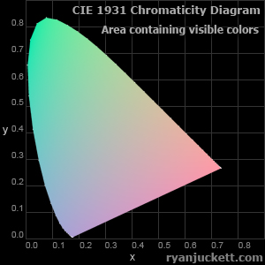
I mentioned earlier that only part of XYZ space corresponds to human-visible color. The area shown in this diagram is the xy representation of that visible range. You monitor isn't capable of displaying all visible chromaticities (unless maybe you are reading this long after I wrote it in which case, awesome!). This is why I haven't bothered to put much color in this image. The subtle color you do see is sort of a compression of all visible chromaticities into RGB space but even that is a bit of a hack and I wouldn't view the displayed chromaticities as anything scientific.
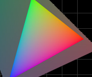
Without getting too off track, if you are familiar with linear algebra or 3D math, you might be wondering what we are actually looking at here spatially (it did all start from some 3D XYZ space after all). When creating the xyz values we essentially made a perspective projection of XYZ space onto the XYZ plane containing the points (1,0,0), (0,1,0), (0,0,1). In doing so, the positive octant of XYZ space all ends up in the triangle created by those three points. Our xy chromaticity diagram is an orthographic view of this three-dimensional triangle along the Z-axis.
Defining an RGB Color Space
Now that we are familiar with XYZ space and xy chromaticity coordinates, we can start using them to define RGB color spaces. This definition consists of xy chromaticity values for the red primary, green primary, blue primary, and white point along with a gamma correction curve. I'll be using the sRGB color space in my examples below. sRGB is the standard color space for the internet and thus your browser should do a pretty good job of displaying it. This actually brings up an interesting example of where color space conversion could be of use. If it is assumed that the internet is all encoded with sRGB color, and you were making some new cell phone that has different display primaries, you would optimally map from sRGB space to the phone's RGB space when browsing the web.
Red, Green and Blue Primaries
Chromaticity coordinates are given for each primary of the display. For sRGB space, they are as follows:
red = \(\begin{bmatrix}0.64 \\ 0.33\end{bmatrix}\)
green = \(\begin{bmatrix}0.30 \\ 0.60\end{bmatrix}\)
blue = \(\begin{bmatrix}0.15 \\ 0.06\end{bmatrix}\)
If you recall from earlier, the gamut of a color space is the subset of color that can be represented by that space. We can now graph the sRGB gamut on our chromaticity diagram. Comparing the listed chromaticity coordinates with the diagram, you'll find they match the corners of the triangular sRGB color gamut.
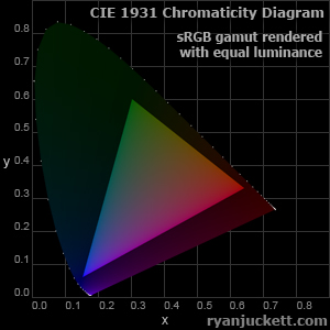
Being the standard color space of the internet (and probably pretty close to your monitor's color space), only chromaticities within that triangle can be created on the web. I have also specifically rendered this image to accurately represent those chromaticities assuming your monitor is properly calibrated (which it probably isn't - mine certainly isn't).
The first time I ever saw one of these diagrams I was a bit concerned, because it looks like our monitors don't come close to handling the color green. Just look at all that visible color to the upper left of the triangle that cannot be displayed! Fortunately, it turns out that things aren't as bad as they look. Both xy and XYZ space are a bit stretched and skewed with respect to how we perceive color. You'll notice a bunch of little dots curving around the diagram in the shape of a tongue. Those dots represent the visible light spectrum in terms of wavelength separated at intervals of 5 nanometers. The details of it are a bit off topic from our goals, but knowing that they have some linear spacing helps us see the distortion in the diagram. The dots travel from red light, through green light, and end at blue light. As you can see, the spacing gets stretched near the greens and very compressed near the blues and reds. Essentially, the error in green color isn't as bad as the diagram makes it seem.
White Point
This might seem a bit odd at first, but the white point is used to specify the color of white. One might expect that the color of white would actually be white, but that is only half true. I say that it's "half true" because perceptually a color may look white, while physically it actually has some color tint. The human vision system is a complex beast and will more or less choose what color should be perceived as white according to what is in view. This color which should be considered as white is known as the white point.
For example, normal incandescent light bulbs give off a red-orange light, while mid-day sun light is closer to a more neutral white. Regardless of this color shift, you perceive a white piece of paper as being white when you look at it under a light bulb or outside on a sunny day. Granted, you may be conscious of the hue shift to some extent, but the point is that you do not get confused thinking that all of your paper turned reddish when you are under a light bulb. Understanding this perceptual effect is actually important in photography. Color correction is often applied to photographs such that the white points which images were captured at are converted to the white points at which images will be viewed at.
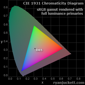
For sRGB, the white point has chromaticity coordinates (0.3127, 0.3290). This white point is also known as D65 which is an estimation of the white color produced by mid-day sunlight. Let's map it on the chromaticity diagram.
Gamma Correction Curve
The gamma correction curve is used to convert pixel luminance from a linear scale to an exponential scale. When encoding the final pixel value, the curve is used to gamma compress linear luminance to a gamma corrected value. When decoding a pixel value, the inverse curve is used to gamma expand the value back to linear units.
We don't perceive the luminance of a color on a linear scale, so this gamma compression actually helps us store more useful information in a limited number of bits per pixel. This nonlinear relationship between linear luminance and the perceived brightness of a color (also known as lightness) is shown below.
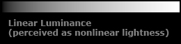
If we were to store image values on a linear scale, single steps in value would correspond to large steps in lightness on the lower end of the scale and minor steps in lightness at the higher end of the scale. As a result, we would lose a lot of lightness fidelity in dark colors.
Now let's look at luminance using the sRGB gamma corrected curve.
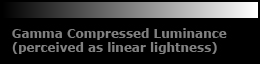
We now get consistent steps of lightness across all values letting us encode lightness with more fidelity across the entire scale. While this image does show linear lightness (human perception), it should be stressed that we are no longer working with linear luminance (physics).
This concept is the source of a lot of lighting errors in older 3D video games (actually a number of new ones still have the problem too). Because of hardware limitations and performance issues, some video games just perform their lighting in the non-linear RGB space that their textures were encoded in. This results in the addition of lights creating brighter results than intended. This is pretty easy to see in the above images. If you locate the pixel with a grey color of (128,128,128) in each scale, you will see that it is around 22% into the linear luminance image and exactly 50% in the gamma corrected image. Now let's say you were adding two lights together at this luminance. In the linear scale you would double your 22% putting you 44% into the linear image which has the correct value of (178,178,178). In the gamma corrected scale you would double your 50% putting you at 100% into the gamma corrected image which has an over-bright value of (255,255,255).
In addition to the benefits of encoding lightness, gamma curves are also chosen to match physical output properties of a display device. For example, the electron guns of a CRT monitor have a non-linear output and must be supplied with gamma corrected input such that the appropriate real-world luminance is created.
A simple gamma correction curve is often defined as \(\mathrm{compressed} = \mathrm{linear} ^ {1 / \gamma}\) where the gamma value, \(\gamma\), is some number greater than 1.0. In the case of sRGB, the gamma curve is a bit more involved. It is built by piecing together two separate curves. Lower input values use a linear curve while higher while higher input values use an exponential curve.
The equations to convert linear sRGB values to gamma corrected sRGB values are
\(C_{\mathrm{srgb}}= \begin{cases}(12.92)C_{\mathrm{linear}}, & C_{\mathrm{linear}} \le 0.0031308\\ (1.055)C_{\mathrm{linear}}^{1/2.4}-0.055, & C_{\mathrm{linear}} > 0.0031308 \end{cases}\)
and the equations to convert gamma corrected sRGB values back to linear sRGB values are
\(C_{\mathrm{linear}}=
\begin{cases}\frac{C_{\mathrm{srgb}}}{12.92}, & C_{\mathrm{srgb}}\le0.04045\\
\left(\frac{C_{\mathrm{srgb}}+0.055}{1.055}\right)^{2.4}, & C_{\mathrm{srgb}}>0.04045
\end{cases}\)
Linear Transformation of Color
We now know how an RGB color space is defined and how to use the gamma curve for converting between linear and gamma corrected values. That leaves us with the final step of converting from a linear RGB color to an XYZ color. Once we are in XYZ space we can convert back to any RGB space of our choosing, but that's really just the beginning. Because XYZ space is a standard color space from which others are defined, we could choose to convert to a number of non-RGB color spaces such as the more perceptually uniform Lab color space or the biologically driven LMS color space.
A fundamental part of the conversion between linear RGB space and XYZ space is recognizing that they are both vector spaces. This basically means that numbers scale in a linear fashion. In contrast, the gamma corrected sRGB space scales luminance in a non-linear manner and is thus not a vector space with respect to luminance. If you've got some sort of math fetish and want to go into more depth on the subject, look up Grassmann's law which talks about color perception as linear combinations.
Knowing that we are working within a vector space puts a whole assortment of linear algebra tools at our disposal. One such tool from linear algebra we will make use of is defining the basis of one color space in terms of another. This is similar to defining the transformation of an object in a 3d space.
As we discussed earlier, an RGB color space is built by adding together three primary colors. The first primary is near the red portion of the spectrum. The second is near green. The third is near blue. To get the color yellow, we add the red and green primary colors together. This operation can be viewed as 3-dimensional vector addition. Let vectors \({\bf i}\), \({\bf j}\) and \({\bf k}\) equal our primary colors red, green, and blue respectively such that
\({\bf i} = \mathrm{red} = \begin{bmatrix}1\\0\\0\end{bmatrix}\ \ \ {\bf j} = \mathrm{green} = \begin{bmatrix}0\\1\\0\end{bmatrix}\ \ \ {\bf k} = \mathrm{blue} = \begin{bmatrix}0\\0\\1\end{bmatrix}\)
We can now define yellow as vector \({\bf i}\) plus vector \({\bf j}\).
\({\bf \mathrm{yellow}} = {\bf i} + {\bf j} = \begin{bmatrix}1\\0\\0\end{bmatrix} + \begin{bmatrix}0\\1\\0\end{bmatrix} = \begin{bmatrix}1\\1\\0\end{bmatrix}\)
The color orange is a combination of the red primary and half of the green primary. This requires us to scale the green primary when we add it to red. The resulting math for orange is
\({\bf \mathrm{orange}} = {\bf i} + 0.5{\bf j} = \begin{bmatrix}1\\0\\0\end{bmatrix} + 0.5\begin{bmatrix}0\\1\\0\end{bmatrix} = \begin{bmatrix}1\\0.5\\0\end{bmatrix}\)
Essentially, any color in a linear RGB space can be built as a linear combination of the \({\bf i}\), \({\bf j}\), and \({\bf k}\) (i.e. red, green, and blue) basis vectors for that space. In more general terms, we can define any color using a red scalar \(r\), green scalar \(g\), and blue scalar \(b\) using the following equation.
\({\bf \mathrm{color}} = r{\bf i} + g{\bf j} + b{\bf k}\)
This might seem like we are over complicating the situation, but it will pay off. First, let's just run through some examples defining colors in this manner.
| color | r | g | b | equation |
| yellow | 1 | 1 | 0 | \(1{\bf i}+1{\bf j}+0{\bf k} = \begin{bmatrix}1\\1\\0\end{bmatrix}\) |
| orange | 1 | 0.5 | 0 | \(1{\bf i}+0.5{\bf j}+0{\bf k} = \begin{bmatrix}1\\0.5\\0\end{bmatrix}\) |
| cyan | 0 | 1 | 1 | \(0{\bf i}+1{\bf j}+1{\bf k} = \begin{bmatrix}0\\1\\1\end{bmatrix}\) |
| red | 1 | 0 | 0 | \(1{\bf i}+0{\bf j}+0{\bf k} = \begin{bmatrix}1\\0\\0\end{bmatrix}\) |
| blue | 0 | 0 | 1 | \(0{\bf i}+0{\bf j}+1{\bf k} = \begin{bmatrix}0\\0\\1\end{bmatrix}\) |
In the examples above, the RGB primaries, i, j and k, were defined with respect to their own RGB color space which made the values fairly trivial. Things become more interesting when we start working with respect to a different color space such as XYZ.
The goal is to find the three XYZ colors that match the primaries of a linear RGB space. Once we have \({\bf i}\), \({\bf j}\), and \({\bf k}\) in XYZ space, we can use the same \(r\), \(g\) and \(b\) scalars to find the XYZ value of an RGB color. I'll be going over how we can derive these new primaries momentarily, but first let's assume we already know their values so we can clarify the process with an example. Let \({\bf l}\) be the red primary in XYZ space, \({\bf m}\) be the green primary in XYZ space and \({\bf n}\) be the blue brimary in XYZ space.
We can now calculate any linear RGB color in XYZ space as a linear combination of the primaries in XYZ space.
\({\bf \mathrm{color}_{\mathrm{XYZ}}} = r{\bf l} + g{\bf m} + b{\bf n}\)
Recalling that orange was defined by the scalars r=1, g=0.5 and b=0, we can calculate the linear RGB color orange in XYZ space like so:
\({\bf \mathrm{orange}_{\mathrm{XYZ}}} = 1{\bf l} + 0.5{\bf m} + 0{\bf n}\)
We can take this whole process one step further by recognizing that we are really multiplying a vector by a transformation matrix to convert it from linear RGB space to XYZ space. In the previous example we were using the XYZ vectors \({\bf l}\), \({\bf m}\) and \({\bf n}\) to build the transformation matrix. Let's specify the three vectors in terms of their components.
\({\bf l} = \begin{bmatrix}l_X\\l_Y\\l_Z\end{bmatrix}\ \ \ {\bf m} = \begin{bmatrix}m_X\\m_Y\\m_Z\end{bmatrix}\ \ \ {\bf n} = \begin{bmatrix}n_X\\n_Y\\n_Z\end{bmatrix}\)
By combing these three column vectors into a column major transformation matrix, we can rewrite our color transformation equation as follows.
\({\bf \mathrm{color}_{\mathrm{XYZ}}} = \begin{bmatrix}l_X & m_X & n_X\\l_Y & m_Y & n_Y\\l_Z & m_Z & n_Z\end{bmatrix}\begin{bmatrix}r\\g\\b\end{bmatrix}\)
Deriving the Transformation Matrices
As shown earlier, the transformation matrix from linear RGB space to XYZ space has columns built from the primary RGB colors in XYZ space. In order to find these values, we need to use the RGB space's xy chromaticity coordinates for red, green, blue, and white. Notice that we only have the x and y coordinates. As discussed earlier, we can compute the z coordinate from x and y but we need either X, Y or Z in order to convert back to XYZ coordinates. As it stands, we don't have enough information to go from xy chromaticity space to XYZ space, but do to the intentions of our transformation, we can make one more assumption.
Let's clarify the purpose of this transformation. I previously mentioned how the eye adapts to the lighting environment to choose what color should be perceived as white. For our purposes we want to consider the perceived white as being maximum luminance. This means that if we transformed from RGB space A into XYZ space and then into RGB space B, we would want the white from RGB space A to maintain luminance in RGB space B. All we need to do is make sure that when an RGB space transforms into XYZ space the white values always ends up with a consistent Y (i.e. a consistent relative luminosity).
I mentioned that choosing any Y luminosity for the white points will do as long as we are consistent, but it is standard practice to use a Y value of 1 for full luminance. Sometimes you may see a Y of 100 used as full luminance, but in this instance a value of 1 is the norm. With a target Y value for white, we now have enough constraints to solve for our matrix. Let's list the variables we start with.
| variable | value | description |
| \({\bf r}_{\mathrm{RGB}}\) | \(\begin{bmatrix}1\\0\\0\end{bmatrix}\) | The linear RGB coordinates of the red primary. |
| \({\bf g}_{\mathrm{RGB}}\) | \(\begin{bmatrix}0\\1\\0\end{bmatrix}\) | The linear RGB coordinates of the green primary. |
| \({\bf b}_{\mathrm{RGB}}\) | \(\begin{bmatrix}0\\0\\1\end{bmatrix}\) | The linear RGB coordinates of the blue primary. |
| \({\bf w}_{\mathrm{RGB}}\) | \(\begin{bmatrix}1\\1\\1\end{bmatrix}\) | The linear RGB coordinates of the while point. |
| \({\bf r}_{\mathrm{xy}}\) | This is defined per RGB space. | The xy chromaticity coordinates of the red primary. |
| \({\bf g}_{\mathrm{xy}}\) | This is defined per RGB space. | The xy chromaticity coordinates of the green primary. |
| \({\bf b}_{\mathrm{xy}}\) | This is defined per RGB space. | The xy chromaticity coordinates of the blue primary. |
| \({\bf w}_{\mathrm{xy}}\) | This is defined per RGB space. | The xy chromaticity coordinates of the white point. |
| \(w_{\mathrm{Y}}\) | \(1\) | The relative luminance value of the white point in XYZ space. |
The goal is to solve for a column-major transformation matrix, \({\bf M}\), that will convert from linear RGB space to XYZ space. The first step is to convert all xy chromaticity coordinates to xyz chromaticity coordinates by using the previously discussed equation \(z = 1 - x - y\).
\({\bf r}_{\mathrm{xyz}}=\begin{bmatrix}r_{\mathrm{x}} \\ r_{\mathrm{y}} \\ 1-r_{\mathrm{x}}-r_{\mathrm{y}}\end{bmatrix}\)
\({\bf g}_{\mathrm{xyz}}=\begin{bmatrix}g_{\mathrm{x}} \\ g_{\mathrm{y}} \\ 1-g_{\mathrm{x}}-g_{\mathrm{y}}\end{bmatrix}\)
\({\bf b}_{\mathrm{xyz}}=\begin{bmatrix}b_{\mathrm{x}} \\ b_{\mathrm{y}} \\ 1-b_{\mathrm{x}}-b_{\mathrm{y}}\end{bmatrix}\)
\({\bf w}_{\mathrm{xyz}}=\begin{bmatrix}w_{\mathrm{x}} \\ w_{\mathrm{y}} \\ 1-w_{\mathrm{x}}-w_{\mathrm{y}}\end{bmatrix}\)
The next step is to define an equation for converting from xyz space to XYZ space. Using the XYZ to xyz equations \(x=\frac{X}{X+Y+Z}\), \(y=\frac{Y}{X+Y+Z}\) and \(z=\frac{Z}{X+Y+Z}\), let's define an XYZ vector \({\bf v}_{\mathrm{XYZ}}\) in terms of its chromaticity coordinates \({\bf v}_{\mathrm{xyz}}\)
\({\bf v}_{\mathrm{xyz}}\ =\ (\frac{v_{\mathrm{X}}}{v_{\mathrm{X}}+v_{\mathrm{Y}}+v_{\mathrm{Z}}},\ \frac{v_{\mathrm{Y}}}{v_{\mathrm{X}}+v_{\mathrm{Y}}+v_{\mathrm{Z}}},\ \frac{v_{\mathrm{Z}}}{v_{\mathrm{X}}+v_{\mathrm{Y}}+v_{\mathrm{Z}}})\)
\({\bf v}_{\mathrm{xyz}}\ =\ \frac{1}{v_{\mathrm{X}}+v_{\mathrm{Y}}+v_{\mathrm{Z}}}(v_{\mathrm{X}},\ v_{\mathrm{Y}},\ v_{\mathrm{Z}})\ =\ \frac{1}{v_{\mathrm{X}}+v_{\mathrm{Y}}+v_{\mathrm{Z}}}{\bf v}_{\mathrm{XYZ}}\)
\({\bf v}_{\mathrm{XYZ}}\ =\ (v_{\mathrm{X}}+v_{\mathrm{Y}}+v_{\mathrm{Z}}){\bf v}_{\mathrm{xyz}}\)
Now we can solve for \({\bf w}_{\mathrm{XYZ}}\) by using our known value of \(w_{\mathrm{Y}}\) and the above conversion from xyz space to XYZ space.
\(w_{\mathrm{y}}=\frac{w_{\mathrm{Y}}}{w_{\mathrm{X}}+w_{\mathrm{Y}}+w_{\mathrm{Z}}}\)
\((w_{\mathrm{X}}+w_{\mathrm{Y}}+w_{\mathrm{Z}})=\frac{w_{\mathrm{Y}}}{w_{\mathrm{y}}}=\frac{1}{w_{\mathrm{y}}}\)
\({\bf w}_{\mathrm{XYZ}} = (w_{\mathrm{X}}+w_{\mathrm{Y}}+w_{\mathrm{Z}}){\bf w}_{\mathrm{xyz}} = (\frac{1}{w_{\mathrm{y}}}){\bf w}_{\mathrm{xyz}}\)
Now we can work towards solving for \({\bf M}\). To do this we first need to recall that the columns of \({\bf M}\) are the red, green, and blue primaries in XYZ space. Let's define \({\bf M}\) using our xyz to XYZ conversion,
\({\bf M} = \begin{bmatrix}{\bf r}_{\mathrm{XYZ}}\ & \ {\bf g}_{\mathrm{XYZ}}\ & \ {\bf b}_{\mathrm{XYZ}}\end{bmatrix}\)
\({\bf M} = \begin{bmatrix}(r_{\mathrm{X}}+r_{\mathrm{Y}}+r_{\mathrm{Z}}){\bf r}_{\mathrm{xyz}}\ & \ (g_{\mathrm{X}}+g_{\mathrm{Y}}+g_{\mathrm{Z}}){\bf g}_{\mathrm{xyz}}\ & \ (b_{\mathrm{X}}+b_{\mathrm{Y}}+b_{\mathrm{Z}}){\bf b}_{\mathrm{xyz}}\end{bmatrix}\)
Expanding our column vector notation we get:
\({\bf M} = \begin{bmatrix} (r_{\mathrm{X}}+r_{\mathrm{Y}}+r_{\mathrm{Z}})r_{\mathrm{x}}\ & \ (g_{\mathrm{X}}+g_{\mathrm{Y}}+g_{\mathrm{Z}})g_{\mathrm{x}}\ & \ (b_{\mathrm{X}}+b_{\mathrm{Y}}+b_{\mathrm{Z}})b_{\mathrm{x}} \\ (r_{\mathrm{X}}+r_{\mathrm{Y}}+r_{\mathrm{Z}})r_{\mathrm{y}}\ & \ (g_{\mathrm{X}}+g_{\mathrm{Y}}+g_{\mathrm{Z}})g_{\mathrm{y}}\ & \ (b_{\mathrm{X}}+b_{\mathrm{Y}}+b_{\mathrm{Z}})b_{\mathrm{y}} \\ (r_{\mathrm{X}}+r_{\mathrm{Y}}+r_{\mathrm{Z}})r_{\mathrm{z}}\ & \ (g_{\mathrm{X}}+g_{\mathrm{Y}}+g_{\mathrm{Z}})g_{\mathrm{z}}\ & \ (b_{\mathrm{X}}+b_{\mathrm{Y}}+b_{\mathrm{Z}})b_{\mathrm{z}}\end{bmatrix}\)
Noticing that each column of \({\bf M}\) is a scalar multiple of the respective xyz primary color, we can factor a scale matrix out of \({\bf M}\) like so:
\({\bf M} = \begin{bmatrix}r_{\mathrm{x}} & g_{\mathrm{x}} & b_{\mathrm{x}} \\ r_{\mathrm{y}} & g_{\mathrm{y}} & b_{\mathrm{y}} \\ r_{\mathrm{z}} & g_{\mathrm{z}} & b_{\mathrm{z}}\end{bmatrix}\begin{bmatrix}(r_{\mathrm{X}}+r_{\mathrm{Y}}+r_{\mathrm{Z}}) & 0 & 0 \\ 0 & (g_{\mathrm{X}}+g_{\mathrm{Y}}+g_{\mathrm{Z}}) & 0 \\ 0 & 0 & (b_{\mathrm{X}}+b_{\mathrm{Y}}+b_{\mathrm{Z}})\end{bmatrix}\)
We know all of xyz primary values and thus know the left matrix in the above equation. Our unknowns are now down to the three scalar values that make up the right matrix. Note that while each of those scalars is written as a sum of X, Y and Z components, we only really care about the summed result and not the individual parts. That is why I say there are only three unknowns instead of nine. In order to solve for the three unknowns, we will use our known RGB and XYZ values of the white point. Because \({\bf M}\) transforms from RGB to XYZ space, we can declare the following equality:
\({\bf w}_{\mathrm{XYZ}} = {\bf M} {\bf w}_{\mathrm{RGB}}\)
\({\bf w}_{\mathrm{XYZ}} = \begin{bmatrix}r_{\mathrm{x}} & g_{\mathrm{x}} & b_{\mathrm{x}} \\ r_{\mathrm{y}} & g_{\mathrm{y}} & b_{\mathrm{y}} \\ r_{\mathrm{z}} & g_{\mathrm{z}} & b_{\mathrm{z}}\end{bmatrix}\begin{bmatrix}(r_{\mathrm{X}}+r_{\mathrm{Y}}+r_{\mathrm{Z}}) & 0 & 0 \\ 0 & (g_{\mathrm{X}}+g_{\mathrm{Y}}+g_{\mathrm{Z}}) & 0 \\ 0 & 0 & (b_{\mathrm{X}}+b_{\mathrm{Y}}+b_{\mathrm{Z}})\end{bmatrix} {\bf w}_{\mathrm{RGB}}\)
Let's substitute in our know the value of \({\bf w}_{\mathrm{RGB}}\).
\({\bf w}_{\mathrm{XYZ}} = \begin{bmatrix}r_{\mathrm{x}} & g_{\mathrm{x}} & b_{\mathrm{x}} \\ r_{\mathrm{y}} & g_{\mathrm{y}} & b_{\mathrm{y}} \\ r_{\mathrm{z}} & g_{\mathrm{z}} & b_{\mathrm{z}}\end{bmatrix}\begin{bmatrix}(r_{\mathrm{X}}+r_{\mathrm{Y}}+r_{\mathrm{Z}}) & 0 & 0 \\ 0 & (g_{\mathrm{X}}+g_{\mathrm{Y}}+g_{\mathrm{Z}}) & 0 \\ 0 & 0 & (b_{\mathrm{X}}+b_{\mathrm{Y}}+b_{\mathrm{Z}})\end{bmatrix} \begin{bmatrix}1\\1\\1\end{bmatrix}\)
Now we can multiply our substituted \({\bf w}_{\mathrm{RGB}}\) vector by the scale matrix.
\({\bf w}_{\mathrm{XYZ}} = \begin{bmatrix}r_{\mathrm{x}} & g_{\mathrm{x}} & b_{\mathrm{x}} \\ r_{\mathrm{y}} & g_{\mathrm{y}} & b_{\mathrm{y}} \\ r_{\mathrm{z}} & g_{\mathrm{z}} & b_{\mathrm{z}}\end{bmatrix}\begin{bmatrix}(r_{\mathrm{X}}+r_{\mathrm{Y}}+r_{\mathrm{Z}}) \\ (g_{\mathrm{X}}+g_{\mathrm{Y}}+g_{\mathrm{Z}}) \\ (b_{\mathrm{X}}+b_{\mathrm{Y}}+b_{\mathrm{Z}})\end{bmatrix}\)
We will now left multiply each side of the equation by the inverse of our remaining 3x3 matrix. This will put all of our known values on the left side of the equation and our unknown values on the right. If you are unfamiliar with calculating the inverse of a 3x3 matrix, I will provide code at the end of the article, but for the sake of sanity won't be writing a full derivation here. Google should bring up a ton of results about the process including this one from Wikipedia and this one from Mathwords.
\(\begin{bmatrix}r_{\mathrm{x}} & g_{\mathrm{x}} & b_{\mathrm{x}} \\ r_{\mathrm{y}} & g_{\mathrm{y}} & b_{\mathrm{y}} \\ r_{\mathrm{z}} & g_{\mathrm{z}} & b_{\mathrm{z}}\end{bmatrix}^{-1} {\bf w}_{\mathrm{XYZ}} = \begin{bmatrix}(r_{\mathrm{X}}+r_{\mathrm{Y}}+r_{\mathrm{Z}}) \\ (g_{\mathrm{X}}+g_{\mathrm{Y}}+g_{\mathrm{Z}}) \\ (b_{\mathrm{X}}+b_{\mathrm{Y}}+b_{\mathrm{Z}})\end{bmatrix}\)
We can now rebuild our RGB to XYZ transformation matrix \({\bf M}\). Multiplying our \({\bf w}_{\mathrm{XYZ}}\) vector by the inverse of the above 3x3 matrix will give us the scalar values which convert the primary xyz coordinates to XYZ coordinates. These are the three unknowns of the scalar matrix that we factored out of \({\bf M}\).
In order to get the matrix transforming in the opposite direction (from XYZ space to linear RGB space), we can use the inverse of \({\bf M}\). We could also derive the matrix in a similar fashion to above, but just using the inverse seems like a simpler approach after this much typing.
Linear Transformation Example for sRGB Space
To help understand the matrix derivation, let's run through the numbers for the sRGB color space. First off, recall the xy chromaticity coordinates of red, green, blue and white that we plotted on the chromaticity diagram.
\({\bf r}_{\mathrm{xy}}=\begin{bmatrix}0.64\\0.33\end{bmatrix}\)
\({\bf g}_{\mathrm{xy}}=\begin{bmatrix}0.30\\0.60\end{bmatrix}\)
\({\bf b}_{\mathrm{xy}}=\begin{bmatrix}0.15\\0.06\end{bmatrix}\)
\({\bf w}_{\mathrm{xy}}=\begin{bmatrix}0.3127\\0.3290\end{bmatrix}\)
Next convert the xy coordinates to xyz coordinates.
\({\bf r}_{\mathrm{xyz}}=\begin{bmatrix}r_{\mathrm{x}} \\ r_{\mathrm{y}} \\ 1-r_{\mathrm{x}}-r_{\mathrm{y}}\end{bmatrix} = \begin{bmatrix}0.64 \\ 0.33 \\ 0.03\end{bmatrix}\)
\({\bf g}_{\mathrm{xyz}}=\begin{bmatrix}g_{\mathrm{x}} \\ g_{\mathrm{y}} \\ 1-g_{\mathrm{x}}-g_{\mathrm{y}}\end{bmatrix} = \begin{bmatrix}0.30 \\ 0.60 \\ 0.10\end{bmatrix}\)
\({\bf b}_{\mathrm{xyz}}=\begin{bmatrix}b_{\mathrm{x}} \\ b_{\mathrm{y}} \\ 1-b_{\mathrm{x}}-b_{\mathrm{y}}\end{bmatrix} = \begin{bmatrix}0.15 \\ 0.06 \\ 0.79\end{bmatrix}\)
\({\bf w}_{\mathrm{xyz}}=\begin{bmatrix}w_{\mathrm{x}} \\ w_{\mathrm{y}} \\ 1-w_{\mathrm{x}}-w_{\mathrm{y}}\end{bmatrix} = \begin{bmatrix}0.3127 \\ 0.3290 \\ 0.3583\end{bmatrix}\)
Next convert our white point xyz coordinate to an XYZ coordinate by using a Y luminance value of 1.
\({\bf w}_{\mathrm{XYZ}} = (\frac{1}{w_{\mathrm{y}}})w_{\mathrm{xyz}} = \frac{1}{0.3290}\begin{bmatrix}0.3127 \\ 0.3290 \\ 0.3583\end{bmatrix} = \begin{bmatrix}0.950455927\\1\\1.089057751\end{bmatrix}\)
Solve for the (X+Y+Z) scalar values that will convert each xyz primary to XYZ space.
\(\begin{bmatrix}(r_{\mathrm{X}}+r_{\mathrm{Y}}+r_{\mathrm{Z}}) \\ (g_{\mathrm{X}}+g_{\mathrm{Y}}+g_{\mathrm{Z}}) \\ (b_{\mathrm{X}}+b_{\mathrm{Y}}+b_{\mathrm{Z}})\end{bmatrix} = \begin{bmatrix}r_{\mathrm{x}} & g_{\mathrm{x}} & b_{\mathrm{x}} \\ r_{\mathrm{y}} & g_{\mathrm{y}} & b_{\mathrm{y}} \\ r_{\mathrm{z}} & g_{\mathrm{z}} & b_{\mathrm{z}}\end{bmatrix}^{-1} {\bf w}_{\mathrm{XYZ}}\)
\(\begin{bmatrix}(r_{\mathrm{X}}+r_{\mathrm{Y}}+r_{\mathrm{Z}}) \\ (g_{\mathrm{X}}+g_{\mathrm{Y}}+g_{\mathrm{Z}}) \\ (b_{\mathrm{X}}+b_{\mathrm{Y}}+b_{\mathrm{Z}})\end{bmatrix} = \begin{bmatrix}0.64 & 0.30 & 0.15 \\ 0.33 & 0.60 & 0.06 \\ 0.03 & 0.10 & 0.79\end{bmatrix}^{-1} \begin{bmatrix}0.950455927\\1\\1.089057751\end{bmatrix}\)
\(\begin{bmatrix}(r_{\mathrm{X}}+r_{\mathrm{Y}}+r_{\mathrm{Z}}) \\ (g_{\mathrm{X}}+g_{\mathrm{Y}}+g_{\mathrm{Z}}) \\ (b_{\mathrm{X}}+b_{\mathrm{Y}}+b_{\mathrm{Z}})\end{bmatrix} \approx \begin{bmatrix}2.088353414 & -0.990629183 & -0.321285141 \\ -1.155287818 & 2.236055332 & 0.049531459 \\ 0.066934404 & -0.245426149 & 1.271753681\end{bmatrix} \begin{bmatrix}0.950455927\\1\\1.089057751\end{bmatrix}\)
\(\begin{bmatrix}(r_{\mathrm{X}}+r_{\mathrm{Y}}+r_{\mathrm{Z}}) \\ (g_{\mathrm{X}}+g_{\mathrm{Y}}+g_{\mathrm{Z}}) \\ (b_{\mathrm{X}}+b_{\mathrm{Y}}+b_{\mathrm{Z}})\end{bmatrix} \approx \begin{bmatrix}0.644360624\\1.191947798\\1.203205256\end{bmatrix}\)
Reconstruct the matrix \({\bf M}\) which transforms from linear sRGB space to XYZ space.
\({\bf M} = \begin{bmatrix}r_{\mathrm{x}} & g_{\mathrm{x}} & b_{\mathrm{x}} \\ r_{\mathrm{y}} & g_{\mathrm{y}} & b_{\mathrm{y}} \\ r_{\mathrm{z}} & g_{\mathrm{z}} & b_{\mathrm{z}}\end{bmatrix}\begin{bmatrix}(r_{\mathrm{X}}+r_{\mathrm{Y}}+r_{\mathrm{Z}}) & 0 & 0 \\ 0 & (g_{\mathrm{X}}+g_{\mathrm{Y}}+g_{\mathrm{Z}}) & 0 \\ 0 & 0 & (b_{\mathrm{X}}+b_{\mathrm{Y}}+b_{\mathrm{Z}})\end{bmatrix}\)
\({\bf M} \approx \begin{bmatrix}0.64 & 0.30 & 0.15 \\ 0.33 & 0.60 & 0.06 \\ 0.03 & 0.10 & 0.79\end{bmatrix}\begin{bmatrix}0.644360624 & 0 & 0 \\ 0 & 1.187536638 & 0 \\ 0 & 0 & 1.203205256\end{bmatrix}\)
\({\bf M} \approx \begin{bmatrix}0.412390799 & 0.357584339 & 0.180480788 \\ 0.212639006 & 0.715168679 & 0.072192315 \\ 0.019330819 & 0.11919478 & 0.950532152\end{bmatrix}\)
If you want the reverse transformation from XYZ to linear sRGB space, use the inverse of \({\bf M}\).
\({\bf M}^{-1} \approx \begin{bmatrix}0.412390799 & 0.357584339 & 0.180480788 \\ 0.212639006 & 0.715168679 & 0.072192315 \\ 0.019330819 & 0.11919478 & 0.950532152\end{bmatrix}^{-1}\)
\({\bf M}^{-1} \approx \begin{bmatrix}3.240969942 & -1.537383178 & -0.49861076 \\ -0.969243636 & 1.875967502 & 0.041555057 \\ 0.05563008 & -0.203976959 & 1.056971514\end{bmatrix}\)
Checking the sRGB specification on color.org, you will find the same values for \({\bf M}\) and \({\bf M}^{-1}\) (rounded to 4 decimal places) listed in equations 1.8 and 1.1 respectively. That makes me feel comfortable that the math was all done correctly and implies we can use this method to generate conversion matrices to and from any linear RGB space.
Writing the Code
For the code example, I'm going to show both the algorithm for generating linear transformation matrices and an example of doing a full transformation between sRGB space and XYZ space. In order to implement other RGB spaces, you only need to implement the appropriate gamma correction curve (which should be simpler than the sRGB one) and supply the chromaticity values for the primaries and white point.
These code samples are released under the following license.
/******************************************************************************
  Copyright (c) 2010 Ryan Juckett
  http://www.ryanjuckett.com/

  This software is provided 'as-is', without any express or implied
  warranty. In no event will the authors be held liable for any damages
  arising from the use of this software.

  Permission is granted to anyone to use this software for any purpose,
  including commercial applications, and to alter it and redistribute it
  freely, subject to the following restrictions:

  1. The origin of this software must not be misrepresented; you must not
     claim that you wrote the original software. If you use this software
     in a product, an acknowledgment in the product documentation would be
     appreciated but is not required.

  2. Altered source versions must be plainly marked as such, and must not be
     misrepresented as being the original software.

  3. This notice may not be removed or altered from any source
     distribution.
******************************************************************************/
First we need a few simple math types.
//******************************************************************************
// 2-dimensional vector.
//******************************************************************************
struct tVec2 { float x, y; };

//******************************************************************************
// 3-dimensional vector.
//******************************************************************************
struct tVec3 { float x, y, z; };

//******************************************************************************
// 3x3 matrix
//******************************************************************************
struct tMat3x3 { float m[3][3]; };
Next we need a few math helper functions.
//******************************************************************************
// Set an indexed matrix column to a given vector.
//******************************************************************************
void Mat_SetCol(tMat3x3 * pMat, int colIdx, const tVec3 & vec)
{
    pMat->m[0][colIdx] = vec.x;
    pMat->m[1][colIdx] = vec.y;
    pMat->m[2][colIdx] = vec.z;
}

//******************************************************************************
// Calculate the inverse of a 3x3 matrix. Return false if it is non-invertible.
//******************************************************************************
bool Mat_Invert(tMat3x3 * pOutMat, const tMat3x3 & inMat)
{
    // calculate the minors for the first row
    float minor00 = inMat.m[1][1]*inMat.m[2][2] - inMat.m[1][2]*inMat.m[2][1];
    float minor01 = inMat.m[1][2]*inMat.m[2][0] - inMat.m[1][0]*inMat.m[2][2];
    float minor02 = inMat.m[1][0]*inMat.m[2][1] - inMat.m[1][1]*inMat.m[2][0];

    // calculate the determinant
    float determinant =   inMat.m[0][0] * minor00
                        + inMat.m[0][1] * minor01
                        + inMat.m[0][2] * minor02;

    // check if the input is a singular matrix (non-invertable)
    // (note that the epsilon here was arbitrarily chosen)
    if( determinant > -0.000001f && determinant < 0.000001f )
        return false;

    // the inverse of inMat is (1 / determinant) * adjoint(inMat)
    float invDet = 1.0f / determinant;
    pOutMat->m[0][0] = invDet * minor00;
    pOutMat->m[0][1] = invDet * (inMat.m[2][1]*inMat.m[0][2] - inMat.m[2][2]*inMat.m[0][1]);
    pOutMat->m[0][2] = invDet * (inMat.m[0][1]*inMat.m[1][2] - inMat.m[0][2]*inMat.m[1][1]);

    pOutMat->m[1][0] = invDet * minor01;
    pOutMat->m[1][1] = invDet * (inMat.m[2][2]*inMat.m[0][0] - inMat.m[2][0]*inMat.m[0][2]);
    pOutMat->m[1][2] = invDet * (inMat.m[0][2]*inMat.m[1][0] - inMat.m[0][0]*inMat.m[1][2]);

    pOutMat->m[2][0] = invDet * minor02;
    pOutMat->m[2][1] = invDet * (inMat.m[2][0]*inMat.m[0][1] - inMat.m[2][1]*inMat.m[0][0]);
    pOutMat->m[2][2] = invDet * (inMat.m[0][0]*inMat.m[1][1] - inMat.m[0][1]*inMat.m[1][0]);

    return true;
}

//******************************************************************************
// Multiply a column vector on the right of a 3x3 matrix.
//******************************************************************************
void Mat_MulVec( tVec3 * pOutVec, const tMat3x3 & mat, const tVec3 inVec )
{
    pOutVec->x = mat.m[0][0]*inVec.x + mat.m[0][1]*inVec.y + mat.m[0][2]*inVec.z;
    pOutVec->y = mat.m[1][0]*inVec.x + mat.m[1][1]*inVec.y + mat.m[1][2]*inVec.z;
    pOutVec->z = mat.m[2][0]*inVec.x + mat.m[2][1]*inVec.y + mat.m[2][2]*inVec.z;
}
These are the gamma correction functions for sRGB color space. These make use of the common run-time library function, powf, from <math.h>.
//******************************************************************************
// Convert an sRGB color channel to a linear sRGB color channel.
//******************************************************************************
float GammaExpand_sRGB(float nonlinear)
{
    return   ( nonlinear <= 0.04045f )
           ? ( nonlinear / 12.92f )
           : ( powf( (nonlinear+0.055f)/1.055f, 2.4f ) );
}

//******************************************************************************
// Convert a linear sRGB color channel to a sRGB color channel.
//******************************************************************************
float GammaCompress_sRGB(float linear)
{
    return   ( linear <= 0.0031308f )
           ? ( 12.92f * linear )
           : ( 1.055f * powf( linear, 1.0f/2.4f ) - 0.055f );
}

//******************************************************************************
// Convert an sRGB color to a linear sRGB color.
//******************************************************************************
void GammaExpand_sRGB(tVec3 * pColor)
{
    pColor->x = GammaExpand_sRGB( pColor->x );
    pColor->y = GammaExpand_sRGB( pColor->y );
    pColor->z = GammaExpand_sRGB( pColor->z );
}

//******************************************************************************
// Convert a linear sRGB color to an sRGB color.
//******************************************************************************
void GammaCompress_sRGB(tVec3 * pColor)
{
    pColor->x = GammaCompress_sRGB( pColor->x );
    pColor->y = GammaCompress_sRGB( pColor->y );
    pColor->z = GammaCompress_sRGB( pColor->z );
}
This function builds the transformation matrix from a linear RGB space to XYZ space,
//******************************************************************************
// Convert a linear sRGB color to an sRGB color
//******************************************************************************
void CalcColorSpaceConversion_RGB_to_XYZ
(
    tMat3x3 *     pOutput,  // conversion matrix
    const tVec2 & red_xy,   // xy chromaticity coordinates of the red primary
    const tVec2 & green_xy, // xy chromaticity coordinates of the green primary
    const tVec2 & blue_xy,  // xy chromaticity coordinates of the blue primary
    const tVec2 & white_xy  // xy chromaticity coordinates of the white point
)
{
    // generate xyz chromaticity coordinates (x + y + z = 1) from xy coordinates
    tVec3 r = { red_xy.x,   red_xy.y,   1.0f - (red_xy.x + red_xy.y) };
    tVec3 g = { green_xy.x, green_xy.y, 1.0f - (green_xy.x + green_xy.y) };
    tVec3 b = { blue_xy.x,  blue_xy.y,  1.0f - (blue_xy.x + blue_xy.y) };
    tVec3 w = { white_xy.x, white_xy.y, 1.0f - (white_xy.x + white_xy.y) };

    // Convert white xyz coordinate to XYZ coordinate by letting that the white
    // point have and XYZ relative luminance of 1.0. Relative luminance is the Y
    // component of and XYZ color.
    //   XYZ = xyz * (Y / y)
    w.x /= white_xy.y;
    w.y /= white_xy.y;
    w.z /= white_xy.y;

    // Solve for the transformation matrix 'M' from RGB to XYZ
    // * We know that the columns of M are equal to the unknown XYZ values of r, g and b.
    // * We know that the XYZ values of r, g and b are each a scaled version of the known
    //   corresponding xyz chromaticity values.
    // * We know the XYZ value of white based on its xyz value and the assigned relative
    //   luminance of 1.0.
    // * We know the RGB value of white is (1,1,1).
    //
    //   white_XYZ = M * white_RGB
    //
    //       [r.x g.x b.x]
    //   N = [r.y g.y b.y]
    //       [r.z g.z b.z]
    //
    //       [sR 0  0 ]
    //   S = [0  sG 0 ]
    //       [0  0  sB]
    //
    //   M = N * S
    //   white_XYZ = N * S * white_RGB
    //   N^-1 * white_XYZ = S * white_RGB = (sR,sG,sB)
    //
    // We now have an equation for the components of the scale matrix 'S' and
    // can compute 'M' from 'N' and 'S'

    Mat_SetCol( pOutput, 0, r );
    Mat_SetCol( pOutput, 1, g );
    Mat_SetCol( pOutput, 2, b );

    tMat3x3 invMat;
    Mat_Invert( &invMat, *pOutput );

    tVec3 scale;
    Mat_MulVec( &scale, invMat, w );

    pOutput->m[0][0] *= scale.x;
    pOutput->m[1][0] *= scale.x;
    pOutput->m[2][0] *= scale.x;

    pOutput->m[0][1] *= scale.y;
    pOutput->m[1][1] *= scale.y;
    pOutput->m[2][1] *= scale.y;

    pOutput->m[0][2] *= scale.z;
    pOutput->m[1][2] *= scale.z;
    pOutput->m[2][2] *= scale.z;
}
Finally, this function just shows an example of converting back and forth between sRGB space and XYZ space.
//******************************************************************************
// Example of using the color space conversion functions
//******************************************************************************
void ExampleColorSpaceConversion()
{
    // define chromaticity coordinates for sRGB space
    tVec2 sRGB_red_xy   = { 0.64f, 0.33f };
    tVec2 sRGB_green_xy = { 0.30f, 0.60f };
    tVec2 sRGB_blue_xy  = { 0.15f, 0.06f };
    tVec2 sRGB_white_xy = { 0.3127f, 0.3290f };

    // generate conversion matrix from linear sRGB space to XYZ space
    tMat3x3 convert_sRGB_to_XYZ;
    CalcColorSpaceConversion_RGB_to_XYZ( &convert_sRGB_to_XYZ,
                                         sRGB_red_xy,
                                         sRGB_green_xy,
                                         sRGB_blue_xy,
                                         sRGB_white_xy );

    // generate conversion matrix from XYZ space to linear sRGB space
    tMat3x3 convert_XYZ_to_sRGB;
    Mat_Invert( &convert_XYZ_to_sRGB, convert_sRGB_to_XYZ );

    // define a color in sRGB space
    tVec3 myColor = { 0.2f, 0.5f, 0.8f };

    // convert form sRGB to XYZ
    {
        // convert from gamma-corrected sRGB to linear sRGB
        GammaExpand_sRGB( &myColor );

        // convert from linear sRGB to XYZ
        Mat_MulVec( &myColor, convert_sRGB_to_XYZ, myColor );
    }

    // convert form XYZ back to sRGB
    {
        // convert from XYZ to linear sRGB
        Mat_MulVec( &myColor, convert_XYZ_to_sRGB, myColor );

        // convert from linear sRGB to gamma-corrected sRGB
        GammaCompress_sRGB( &myColor );
    }
}
Comments